How to read this walk-through. The paper is long (40 pages) and has three layers: the geometry of the rules, which does not depend on the strategy (sections 1–3 of this walk-through), the results for the author's specific strategies (section 4) and the seller model (section 5). The first layer is the most reliable and the most useful. The discrepancies found in our check are in section 6; almost all of them are in the text of the abstract and the conclusions, not in the tables.
Main thesis
A retail prop evaluation has two stages, and the rules reward opposite behavior at each of them. In the evaluation a fast, uneven tempo and large size pay off: the lower limit updates only at the day's close, and the risk is capped by the price of an attempt. On the funded account the same tempo kills: you have to survive a minimum number of days and the consistency rule. Because of this, passing the evaluation says little about skill on its own, and a participant with no edge at all can pass it in roughly 40 % of cases by size selection alone. By Topstep's published data, 16.8 % of accounts pass the evaluation.
The second thesis is about money. At the three firms studied, the break-even win rate at a 1:1.5 ratio lies 0.5–3.6 pp above 40 %, the coin's rate. None of the strategies the author tested over three research cycles reached even zero per trade after costs.
The third thesis is about the seller: its margin is bounded by the gap between how buyers estimate their chances and the true chances. Hence the prediction that it pays to make a soft, visible evaluation and a hard, opaque payout stage. The firms' disclosures fit this: the pass rate is published often, the payout rate by almost nobody.
1. How the product and the model work
Three firms are studied in detail: Lucid Trading, Tradeify, TopOne Futures; a fourth, Apex Trader Funding, is added in section 12.6 as an extreme case on price. Everything is on a 50K account: target , loss limit , trailing the balance high at the day's close. Intraday the balance may drop below the previous peak as long as it stays above .
Price is not cost
| Account (50K) | Price | Activation | Cost to funding | Consistency | Daily limit |
|---|---|---|---|---|---|
| Lucid Flex, evaluation | $98 | none | $98 | none | none |
| Tradeify, evaluation | $87 | none | $87 | 20 % | $1,250 |
| TopOne Elite Access, evaluation | $39 | $189 | $228 | 40 % | none |
| Lucid Direct, funded from the start | $364 | none | $364 | 20 % | $1,200 |
| TopOne InstantSim, funded from the start | $407 | none | $407 | 20 % | $1,250 |
Table 4 of the paper. The cheapest account by advertised price ($39) turns out to be the most expensive in fact ($228) because of the activation fee.
The model
What this is. The result of each trade net of costs is random, with mean and spread ; trades are made per day. The evaluation is passed if at some close the profit is at least , before the balance has dropped to (peak at close − ). The horizon is 90 trading days.
What each symbol means. (mu): the average net result of one trade in dollars. (sigma): the spread of one trade's result in dollars, in effect the position size. : trades per day. : “skill per trade”, the ratio of edge to size.
Two formulas everything else rests on
For a fixed barrier and continuous observation with no drift, the probability of reaching the target before the limit is
This is the same quantity that Villahermosa (2026) writes as . It depends only on the ratio of target to limit. Table 2 of the paper shows that firms make this ratio worse on larger accounts: 0.400 on 25K and 50K, 0.333–0.368 on 100K, 0.308–0.357 on 150K. The bigger the account, the smaller the chance without an edge.
For fixed barriers with a drift of per day and a variance of per day:
What this is. The classic gambler's ruin formula for Brownian motion with drift.
Step by step on the paper's numbers. Cell : , , . Then , , and . The paper has 0.871.
Why this matters. It is an upper bound: a trailing barrier is always worse than a fixed one. How much worse, the author measures by simulation.
| Cell | Fixed barrier, formula | Trailing, simulation | Loss |
|---|---|---|---|
| (5, 100, 10) | 0.871 | 0.731 | −14.0 pp |
| (10, 150, 5) | 0.841 | 0.691 | −15.0 pp |
| (2, 80, 20) | 0.746 | 0.580 | −16.6 pp |
Table 5 of the paper. Our check: the formula gives 0.871 / 0.841 / 0.746 in all three cells; our own simulation of the trailing barrier with no horizon limit gives 0.731 / 0.691 / 0.580, that is, it matches to the third decimal. With a 90-day horizon the probabilities are lower by another 3–5 pp (0.684 / 0.659 / 0.549): in this table the author compares without a horizon, and that is correct, otherwise the loss from the trailing barrier would be mixed up with the loss from running out of time.
2. The main mechanisms
Size can buy a pass with no skill at all
At , that is, with no edge, optimal size selection gives a pass probability of 0.36–0.47, higher with more frequent trading. The mechanism: at a huge size every day ends either above the target or below the limit, and the daily close jumps over the barrier, so the game turns almost into a single coin flip with a chance of about one half.
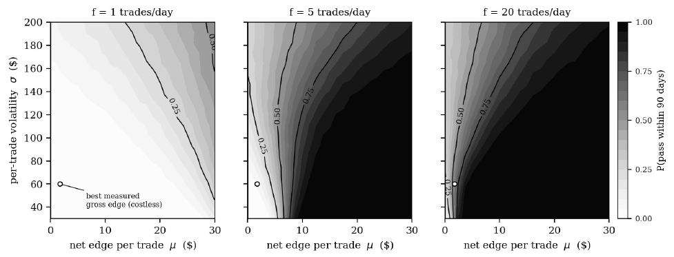
How to read it. Horizontally, the net edge per trade in dollars; vertically, the size in dollars. Darker means a higher probability of passing within 90 days. The white circle: the best gross edge the author measured anywhere, $1.74 at , drawn as if there were no costs.
What to notice. At one trade a day almost the whole figure is light: to pass with probability 0.5 you need $31–34 net per trade. At five trades $5.4–5.8 is enough, at twenty $2.0–3.4 (table 6). The circle lies in the light zone everywhere.
The practical takeaway. The required edge per trade falls sharply with frequency (from $31–34 at one trade a day to $5.4–5.8 at five), but costs per trade do not depend on frequency. These are the “scissors”: frequent trading lowers the edge requirement and at the same time multiplies costs.
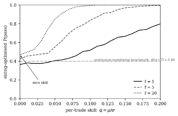
How to read it. Horizontally, skill ; vertically, the pass probability at the best size. The dash-dot line at 0.40 is .
What to notice. The left edge, : about 0.37, 0.43 and 0.47. At five and twenty trades a day this is above 0.40, because daily observation lets the barrier be jumped; at one trade a day it is slightly below. At one trade a day the curve is almost flat up to : skill adds almost nothing to what size gives.
The practical takeaway. A pass does not separate a skilled trader from an unskilled trader who takes large risk.
Skill and size weigh the same
| , best size | , best size | , | , | , | |
|---|---|---|---|---|---|
| −0.04 | 0.322 | 0.378 | 0.000 | 0.021 | 0.035 |
| 0.00 | 0.370 | 0.434 | 0.000 | 0.101 | 0.263 |
| 0.02 | 0.373 | 0.449 | 0.001 | 0.190 | 0.488 |
| 0.05 | 0.409 | 0.554 | 0.002 | 0.394 | 0.774 |
| 0.08 | 0.449 | 0.749 | 0.004 | 0.630 | 0.928 |
| 0.12 | 0.578 | 0.914 | 0.011 | 0.876 | 0.987 |
Table 7 of the paper. At five trades a day and a fixed size, going from zero to a real edge of raises the probability from 0.101 to 0.394, by 29 points. Going from a fixed size to the best size at zero skill raises it from 0.101 to 0.434, by 33 points. The arithmetic adds up. Even a participant with a negative edge () passes in 32–38 % of cases with size selection.
The evaluation needs speed, the funded account slowness
| Trades per day | Evaluation pass at 40 % winners | Days to outcome | Funded-account payout at 40 % |
|---|---|---|---|
| 1 | 23.4 % | 11.4 | 34.8 % |
| 5 | 24.9 % | 3.6 | 23.4 % |
| 20 | 25.4 % | 1.6 | 3.9 % |
Tables 10 and 11 of the paper, combined by us into one. In the evaluation frequency is almost free: the limit updates once a day, and intraday trades do not move it. On the funded account, twenty trades a day over five required days give a hundred chances to touch the floor. Twenty trades at both stages: . Fast in the evaluation and slow afterwards: . Recount: the ratio is 8.9, the author calls it ninefold.
The 20 % consistency rule cuts the payout in half with an uneven profile (34.8 % → 17.4 % in table 3) and costs almost nothing with an even one: one trade a day, the best day about 18 % of the cycle profit. It hits exactly the behavior that helps pass the evaluation.
3. Break-even
What this is. The expected result of one purchased evaluation.
What each symbol means. (pi): the probability of passing the evaluation. (beta): the probability of receiving a payout on the funded account. : the payout size, $1,000 in section 7 of the paper (half of the $2,000 limit). Cost to funding is taken from table 4.
A worked example on the paper's numbers. Section 3.7: at a price of $98 and a published pass rate of 10–20 %, one funded attempt costs $490–980, while the payout is capped at $1,000. Even if the payout is guaranteed, the purchase barely pays for itself.
| Account | Break-even win rate at 1:1.5 | Above the coin (40 %) |
|---|---|---|
| Lucid Flex (no consistency) | 40.9 % | +0.9 pp |
| Tradeify (20 %) | 40.5 % | +0.5 pp |
| TopOne Elite Access (40 %) | 43.6 % | +3.6 pp |
Table 13 of the paper. Our check: our own implementation of the two-stage model, following the description in section 7.1 and the parameters from the repository (risk $250 per trade, costs $5 per trade, five trades a day in the evaluation, one afterwards, withdrawal $2,000, payout $1,000, 60 days), gives 40.90 / 40.51 / 43.55 %. A match to the hundredth. The payout rate at the Lucid Flex break-even point is 0.345, in the paper 34.6 %.
The paper also has a second, earlier implementation of the same calculation, which produced table 12 (expectation by win rate). It is not in the repository, and our implementation does not reproduce it: at 44 % we get +157 / +174 / +27 dollars, table 12 has +106 / +38 / −24. That is legitimate: the two implementations differ in details, and the author says so. The problem is how the result of the two implementations is restated in the abstract (section 6).
4. What was measured on strategies
Three research cycles, about two dozen mechanisms, each with a named “forced counterparty”. The selection gates were set in advance: drawdown against the limit, net edge against costs, an out-of-sample Sharpe of at least 1.5, at least 30 out-of-sample trades. The sample boundary of 7 September 2021 did not move. Costs were included from the first run: of 576 opening range breakout variants, 190 survived without costs and zero with costs.
Costs on the micro contract are 1.12 points per round turn, $2.24. The best gross edge across the cycle II geometries is +0.32 points, that is $0.64 per trade. All ten geometries are negative after costs (appendix C, the best is −$2.37 per trade per contract; that appendix uses costs of $3.00 per round turn from early runs, not the final $2.24).
The two strategies closest to success (a short position into leveraged ETF rebalancing, out-of-sample Sharpe 3.07 on 60 trades; “holiday eve”, 3.15 on 53) pass the gates but give about 19 trades a year between them. A $3,000 target within the limited evaluation horizon is unreachable at that frequency. The author states the result carefully: the measured set contains no edge compatible with the tempo, drawdown and daily limits of the evaluation, which is not the same as “edges do not exist”.
Adversarial test: the rules of a well-known practitioner
A fully formalized rule set of “the most visible public practitioner” (not named; entry on a momentum candle), 324 in-sample configurations, one out-of-sample check. Out of sample: 1,217 trades, 38.54 % winners, −$32.14 per trade. The practitioner claims 57.5 %.
| Account | Pass | Payout | Expectation per account | |
|---|---|---|---|---|
| Lucid Flex | rules | 15.25 % | 16.16 % | −$24.06 |
| coin | 20.50 % | 12.50 % | −$21.12 | |
| TopOne | rules | 15.25 % | 16.16 % | −$152.63 |
| coin | 20.50 % | 12.50 % | −$149.64 |
Part of table 19. The coin passes the evaluation more often than the strategy. The joint probability is 2.46 % for the strategy and 2.56 % for the coin.
What the recount shows, our calculation. The expectation in table 19 adds up only with a payout of : . Section 7 uses a $1,000 payout. The assumption favors the participant and does not change the conclusion, but the text does not state it. The pass and payout probabilities in table 19 are the same for all three firms, although their rules differ: only the price differs. In the TopOne row, the break-even and expectation columns at $3,000 do not agree with each other: the first corresponds to a price of $223.7, the second to $226.5, while table 4 gives a price of $228. The difference is about $3 and does not affect the conclusion.
External check
Topstep publishes statistics for 2025: 16.8 % of accounts completed the evaluation, 51.8 % of people reached funding at least once, 33.3 % of funded traders received a payout, and 0.71 % reached a live-capital account. MyFundedFutures publishes 28.6 % receiving a payout. The author's model gives 34.8 % (table 3) and 34.6 % (solver). For comparison: FPFX, 300,000 accounts at 10 firms: 14 % pass, and 45 % of those receive a payout.
The author sorts out the denominators without being prompted: Topstep's pass rate is per account and its payout rate per person, and multiplying them, as the author did in an earlier version, is not valid. Per person it comes to about 17 %.
5. The seller model
If the seller collects the fee and pays out only payouts, its margin per account is . A zero-sum game. A buyer with correct expectations would buy only when , and there would be no business. So the business exists only where the buyer's expectations () are above the real ones:
What this is. The seller's margin cannot exceed the “expectations gap” multiplied by the payout.
What each symbol means. A hat over a letter means the buyer's estimate at the moment of purchase. (kappa): the price.
Step by step. The buyer buys if . Substitute this into and you get the inequality.
Where this breaks. The model has no operating costs for the seller, no customer acquisition and no other revenue. The author notes this and writes that the expectations gap is not measured:
"The proposition is therefore a constraint on any explanation of the industry's economics rather than a measurement of them".
Hence the prediction: the buyer learns the pass rate quickly and discusses it with others, but learns the payout rate late and alone. It pays the seller to make the evaluation soft and visible and to hide the difficulty in the payout stage. Apex is exactly that: the softest evaluation in the industry and all the restrictions after it (a $2,100 safety buffer, five days with a minimum profit, 50 % consistency, a contract limit three times smaller). Of the ten statistics sources in table 21, eight give a pass rate. Three firms publish a payout rate themselves, and two more sources are cross-firm.
The hedged pair
Buy two accounts, long on one and the same position short on the other. One will reach the target, the other will blow up. A simulation on 200,000 paths: the probability of getting at least one funded account is exactly twice as high, and the price is also twice as high, so the cost of one funding matches to three significant figures ($465 / $314 / $332 / $292 / $267; our recount gives the same numbers). Unequal sizes of 4:1 cut the cost by 17 %. With the real $1,000 payout cap the pair earns $9 on $196 invested, and with 20 % consistency it loses $93. The work is done by the payout cap, not by the ban on hedging.
6. What is shaky in the paper
What the author admits
The author makes many honest caveats, and that is a strength of the paper. Break-even is conditional and depends on the account. The research log and the agent system are not open, and the system was not working at the time of writing. The 88 closed studies are not independent, and there is no multiple-testing correction. The external payout rate rests on two numbers. The expectations gap is not measured. The seller model does not describe a real firm. The hedged pair with imperfect mirroring and with the risk of detection is worse than in the simulation. Corrections to earlier versions are written into the text (a wrong contour in table 6, intraday instead of daily trailing, a wrong bound in proposition 3), with a note on which way each shifts the conclusion.
What our check turned up
1. The break-even range in the abstract and conclusions does not agree with table 13. Abstract: "break-even lies between a 40.5% and 41.5% win rate at 1:1.5 net of costs across the three accounts studied in detail and the two implementations". In table 13 the third of those three accounts, TopOne, has 43.6 %, and we reproduced that value (43.55 %). By table 12 of the same paper, the zero crossing is about 44.7 % for TopOne and about 42.5 % for Tradeify. The 40.5–41.5 % range is correct only for the two cheap accounts. The same wording is repeated in section 14.
2. “41.5 %” for Lucid Flex is not found in any table. Section 7.1: "The independent solve returns 40.9% on Lucid Flex against the 41.5% reported above". Earlier in the text 41.5 % appears only in words; table 12, the only one with results from the first implementation, crosses zero for Lucid Flex between 40 % (−$10) and 42 % (+$42), at 40.38 % by linear interpolation and at 40.42 % by a parabola through three points. Our calculation.
3. Section 11.1 contradicts section 7. "approximately +1.4 percentage points is needed at a ratio of 0.5, against approximately +5 points at 1.5". At 1:1.5 section 7 gives +0.5…+3.6 pp, and the author warns in section 7.1 that the 4–6 pp figures from the author's working notes are not break-even values: "Neither is a break-even". Section 11.1 repeats exactly the withdrawn figure.
4. The comparison with the external payout rate is described incorrectly. "Our figures sit between the two and within six points of both". The model gives 34.8 % and 34.6 %; the published figures are 33.3 % and 28.6 %. Both model figures are above both published ones, not between them, and one of them is 6.2 pp away from 28.6 %. The conclusion “the model is close to the published figures” holds for Topstep (1.5 pp), but not in the way it is written.
5. The “pass without skill” range is given in different ways. In sections 1.2 and 5.3 "roughly 0.36 to 0.47", in section 9.1 "our simulated 28–41%". Figure 2 gives roughly 0.36–0.47 at the left edge, and table 7 gives 0.370 and 0.434 for one and five trades. Where the 28 % in section 9.1 comes from is not said.
6. The “ten standard errors” come from mixing units. Section 10: "each sits roughly ten standard errors above zero". The Sharpe ratios of 3.07 and 3.15 are annual (as stated in section 2.3). Ten standard errors come out if they are treated as per-trade Sharpe: . The author's open script (robustness_and_extensions.py) does exactly that. Converted to a per-trade Sharpe at the frequency the author gives (about 19 trades a year for the two strategies, that is, roughly 9.5 for each), the per-trade Sharpe is about 1.0, and the t-statistics are 7.7 and 7.4, or 6.3 and 6.0 with the non-normality correction. The author's conclusion (above the expected maximum over 127 null trials, about 2.6) still holds, but the margin is noticeably smaller. Our calculation.
7. The conclusions keep a claim withdrawn in section 9.4. Section 14: "the convergence of inverted rule architectures on comparable outcomes". Section 9.4: "It does not establish a conserved joint rate across firms or denominators; §9.3 explains why that stronger claim, made in an earlier draft, does not survive."
What is actually not there, checked. The phrase "hence 7% of buyers paid" (section 9.3), with inputs of 14 % and 45 %, gives 6.3 %, but with the inputs rounded to whole percents the product lies in 6.0–6.6 %, so this is not a discrepancy. Table 8 (days per pass) recomputed: with an early exit after a limit breach we get 265 and 162 days against 264 and 162 in the paper. The script verify.py uses a different formula (each failed attempt counts as the full 90 days) and gives 301 and 175, but the table in the paper is computed correctly. All arithmetic relations in tables 22–26 add up.
Methodological remarks, ours
Table 19 counts the payout as $3,000 rather than $1,000 and uses identical probabilities for three firms with different rules; neither is stated. The research log is closed, so section 8, that is, the conclusion “no strategy passed”, cannot be checked; the tables of sections 4–7 and 12 do not depend on it and are reproducible. Choosing “the rules of the most visible practitioner” without naming them does not let the reader check that the formalization is right; the author admits that the practitioner claims a discretionary overlay.
7. What follows in practice
Passing an evaluation proves skill neither to the seller nor to the trader. If a strategy passes the evaluation, that is compared with a coin of the same size on the same rules, not with zero. Without such a control the pass rate, in the author's words, cannot be interpreted, and that is hard to argue with.
Two stages need two configurations. Fast and large in the evaluation, slow and even on the funded account. Keeping the same tempo at both stages costs roughly a ninefold drop in joint probability.
Look at the cost to funding, not at the price. The activation fee, monthly renewal, resets and the payout cap change the expectation more than the win rate does within a reasonable range.
The break-even threshold is close to the coin, and that is bad news, not good news. Only 0.5–3.6 pp above 40 % at 1:1.5 is needed, but these are net percentages after costs, and costs on a micro contract eat any edge smaller than 1.12 points per trade.
The hedged pair gives nothing with a $1,000 cap and is explicitly banned by the rules of all the firms studied.
8. Testable ideas
| No. | Idea | Type | Where to compute |
|---|---|---|---|
| 1 | Report any strategy result on prop-firm rules next to a coin of the same size run through the same pipeline; a pass rate without a control cannot be interpreted | acceptance metric | Python |
| 2 | Two configurations for two stages: in the evaluation, frequency and size tuned for the pass; on the funded account, one trade a day for the minimum days and consistency; compare the joint probability with a single configuration | design change | Python |
| 3 | Compute the “cost to funding” including activation, renewal and resets for every candidate firm before choosing; the advertised price can differ from it by a factor of 2+ | diagnostic | any |
| 4 | Measure how much pass probability the trailing drawdown eats compared with a fixed one on our trade distributions (in the paper 14–17 pp on Gaussian ones) | diagnostic | Python |
| 5 | Check whether the strategy's gross edge covers costs on the micro contract (≈1.12 points per round turn for the author); on the full contract the fixed commission, according to the author, is proportionally about 10 times lighter, while slippage in points is the same | audit | Python |
| 6 | For each consistency setting (none / 40 % / 20 %) measure the strategy's best-day share of the cycle profit; at a share of about 18 % the 20 % rule is almost free, with an uneven profile it cuts the payout in half | acceptance metric | Python |
| 7 | Convert annual Sharpe to per-trade Sharpe before any correction for the number of trials: ; t-statistic , and with the non-normality correction divide further by | audit | Python |
| 8 | Compare the target-to-limit ratio across account sizes of one firm before buying: at 100K–150K the ceiling for a participant with no edge is 0.31–0.37 against 0.40 at 50K | diagnostic | any |