How to read this walk-through. There are two formulas here, both taken apart in words and on numbers. The main conclusion is in the section «The method in one line», and the most interesting part is the sixth section: it shows where the paper's headline result fails a recount.
1. How the test is built
The question is the same as in Villahermosa's barrier model, but the approach is the reverse. Instead of deriving the probability of passing from the geometry of the rules, the author takes a deliberately meaningless strategy, runs it through one firm's programmed rules and looks at what happens to the money.
From the outset the paper separates two quantities that are constantly confused in this subject.
Simulated result versus real one. The profits and losses on the account determine whether the evaluation is passed, whether the account is alive and whether a payout is due. That is simulated money. The client's real cash flow consists of exactly two things: he pays a subscription and he receives payouts. The economic result is payouts minus account costs, not the change in the simulated balance.
An important consequence for reading follows. Trade commissions are debited from the simulated balance and affect the probability of passing, but they are not a real expense to the client. So they are not part of the $+1,490 net result, and that is methodologically right. The author's wording is misleading here: "the modeled proprietary framework generated +\$1,490.19 of mean net economic P&L per account after account-related costs and trading costs were incorporated". In fact , and there are no trading costs in that difference.
The Topstep rules that are programmed
| Simulated result | Real cash flow |
|---|---|
| Evaluation target: $3,000 | Account cost: $85 a month |
| Maximum loss limit $2,000; trails the balance high | Payout cap: $6,000 per request |
| Evaluation consistency: the best day at most 50 % of the profit needed to pass | Maximum request: 50 % of the profitable balance |
| Daily loss limit: $1,000 | Minimum request: $125 |
| Reset credit: on a failure it lets you shift the charge by 30 days instead of buying the account again | Profit split: 90 % to the client, 10 % to the firm |
| Payout requirement: at least three trading days with at least one trade | |
| Consistency at the funded stage: no day may give more than 40 % of the cycle's profit |
The strategy
- Instrument: Micro E-mini Nasdaq-100 (MNQ)
- Size: 8 contracts
- Frequency: one trade per qualifying day
- Entry: 10:00 New York time
- Direction: randomly long or short with equal probability
- Stop: 100 ticks (25 index points)
- Target: 100 ticks, a 1:1 ratio
- Dollar value of target and stop: ±$400 gross on 8 MNQ
- Costs: $1.22 per round turn per contract, that is $9.76 on a trade of eight
- Time exit: barriers not touched are closed at 16:00
- Session filter: holidays, shortened days and days with no 10:00 bar are excluded
- Ambiguous observations: days where target and stop are both touched within one minute are excluded
A check on the dollar arithmetic. An MNQ tick is 0.25 index points and $0.50 per contract. A hundred ticks is 25 points, that is $50 per contract. On eight contracts, $400. It adds up.
Excluded were 87 shortened holiday days, one day with no 10:00 bar and four days where target and stop were touched within one minute, which came to 0.16 % of 2,485 trades.
A caveat from the author worth reading carefully. Ten thousand paths are not ten thousand independent ten-year market histories. Every simulation uses the same 2,485 historical days and randomises only the direction on each date. The exercise measures how different sequences of trades change the outcome within the observed sample, and does not claim to represent every possible future path. The author states this caveat himself, and below it turns out to be the key to the whole critique.
2. The method in one line
What this is. The entire economic part of the paper. The simulated balance does not enter it at all: it only determines whether matters get as far as a payout.
Step by step. Add up all payouts received. Subtract everything paid for subscriptions and account purchases.
A worked example on the paper's numbers. Payouts $9,368.50, account costs $7,878.30, net result $+1,490.20.
And here is the second formula, the one the paper was written for, and also its most vulnerable point:
Step by step. Divide payouts by costs. Multiply the current subscription price by that ratio.
A worked example on the paper's numbers. . Then , and the account is «$16 cheaper than its fair price».
Why the arithmetic adds up. Account costs of $7,878.30 at an $85 subscription mean 92.69 paid months, which is exactly 61.68 renewals plus 31.01 evaluation purchases. Raise the price to $101.08 and the same 92.69 months cost $9,368, that is, exactly the sum of payouts. Internally the calculation is correct.
What it leaves out. That the price is set not by this strategy but by the whole client population.
3. The base strategy: is it really zero
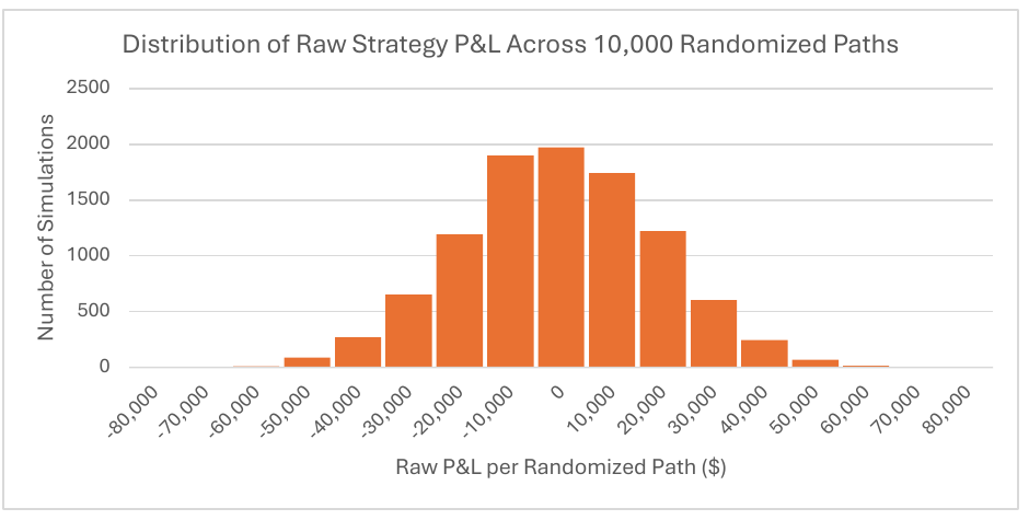
How to read it. Horizontally, the result of one randomised path in dollars, from −$80,000 to +$80,000. Vertically, how many of the ten thousand paths fell into that bin. The distribution is roughly normal and centred near zero, slightly to the left.
What to notice. The symmetry and the centre at zero. That is the proof that the strategy really has no edge: direction was chosen by a coin, and the outcome of one path is decided by whether the coin was kind.
The practical takeaway. The spread is enormous relative to the centre: a path can end at −$50,000 and at +$50,000 with zero expectation. It is precisely this dispersion that is the raw material from which the prop account's «value» is later made.
The base strategy's numbers:
| Quantity | Value |
|---|---|
| Mean number of target wins | 1,143.98 |
| Mean number of stop losses | 1,145.02 |
| Time exits | 196 |
| Win rate among barrier-resolved trades | 49.98 % |
| Mean gross result per trade | −$0.1678 |
| Mean gross result per path | −$416.86 |
| Median per path | −$568 |
| Costs per path (2,485 × $9.76) | −$24,253.60 |
| Net result of the standalone strategy | −$24,670.46 |
The check adds up: , the win rate , and against the stated −$416.86.
The five-year split. The first period (August 2016 to August 2021, 1,246 days): win rate 49.99 %, −$0.0408 per trade, −$50.78 per path. The second (August 2021 to August 2026, 1,239 days): 49.96 %, −$0.2955 per trade, −$366.08 per path. The two periods sum to −$416.86 and match the full sample.
4. The same strategy inside Topstep's rules
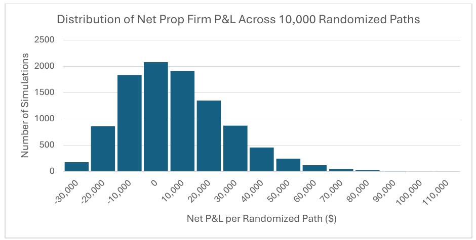
How to read it. Horizontally, the net economic result of one path, from −$30,000 to +$110,000. Vertically, the number of paths. Compare with the previous figure: there the scale is symmetric, here the left edge is cut and the right one is long.
What to notice. The right skew. The mass still sits near zero, but the left tail is cut short. That truncation on the left is the mechanics of the product: the client cannot lose more than he paid in subscriptions.
The practical takeaway. The positive mean does not come from the strategy having got better. It is the same strategy. It comes from the loss distribution being truncated while the profit distribution is not.
| Quantity | Value |
|---|---|
| Mean payouts to the client | $9,368.50 |
| Mean account costs | $7,878.30 |
| Mean net | +$1,490.19 |
| Median net | +$1,036.83 |
| Payout-to-cost ratio | ≈ 1.19 |
| Standard deviation | $3,926.12 |
| 5th / 95th percentile | −$3,995.42 / +$8,612.82 |
| Share of profitable simulations | 60.30 % |
The account life cycle is active rather than reduced to a few lucky payouts: on average per simulation there are 31.01 evaluation purchases, 61.68 renewals, 56.31 reset credits used, 17.62 evaluations passed, 17.47 funded-account failures and 14.95 payouts.
Why several rules turned out inoperative. A daily loss limit of $1,000 is unreachable if target and stop do not exceed $400 and there is one trade a day. Evaluation consistency (the best day at most 50 % of the $3,000 target, that is, at most $1,500) is unreachable for the same reason. The author says so honestly: the system's parameters were chosen with Topstep's rules in view, and $400 is not an optimised value but one that sat conveniently below the daily limit and nullified several rules.
From which comes the first of the paper's two substantive conclusions, and it is a good one:
Prop-firm rules screen out position-sizing behaviour, not trading skill. A fixed size makes part of the rulebook inoperative, and that is not a loophole but a property of the design: the rules are written against a person who scales up after a run, not against one who never changes size at all.
5. The five-year split, where it all breaks
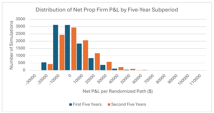
How to read it. The same axes as the previous figure, but two sets of bars: one is the first five-year block (2016 to 2021), the other the second (2021 to 2026).
What to notice. The earlier bars are shifted left relative to the later ones. In the −$10,000 bin the earlier one is taller, and in the bins from +$10,000 rightwards the later one is taller almost everywhere. The later distribution is shifted into the positive as a whole.
The practical takeaway. These are two different businesses, not one with noise. The first five years give a negative median, the second a positive one, while the account rules and the subscription price did not change.
| Quantity | 2016–2021 | 2021–2026 |
|---|---|---|
| Mean net | +$253.08 | +$913.49 |
| Median net | −$214.23 | +$403.34 |
| Share of profitable simulations | 46.45 % | 56.05 % |
| Payouts | $4,155.81 | $5,108.40 |
| Account costs | $3,902.73 | $4,194.91 |
| Payout-to-cost ratio | 1.06 | 1.22 |
| Time exits per path | 196 | 0 |
In the first five years the median is negative and most paths lose money. A positive mean alongside a negative median is pure skew: it is a minority of paths, the ones that ran far to the right, that does the work.
The author's explanation about time exits. In the first block an average of 196 trades per path reached neither target nor stop and were closed at 16:00; in the second there were none at all. More time exits means more trades with a small result in absolute terms, and if an account takes longer to pass or to fall over, it pays for more subscriptions with no increase in the chance of a payout.
The explanation is correct, but the author stops exactly where the main point begins.
6. What does not add up in the paper
6.1 The barrier is fixed in points while the index rose fivefold
Here is the source of the difference between the five-year blocks, and it is not named in the paper once.
Target and stop are set as 25 index points. Over the period the Nasdaq-100 rose from about 4,800 to 24,000. So one and the same «unchanged» barrier meant:
| Moment | Index level | 25 points as a percentage |
|---|---|---|
| 2016 | ≈ 4,800 | 0.52 % |
| 2026 | ≈ 24,000 | 0.10 % |
This is not one strategy across two market regimes. These are two different strategies: in 2016 it risked half a percent of the index, in 2026 one tenth. Hence the zero time exits in the second block: a six-hour session touches a 0.1 % barrier practically always, a 0.52 % barrier far from always, in 15.7 % of cases (196 out of 1,246) it did not.
The author attributes the difference between the periods to the market: "showing that value fluctuates between different market regimes". In fact what fluctuates is not the market but the tested construction itself, because its single parameter is normalised neither to price nor to volatility. For comparison: Villahermosa's barrier model runs into the same effect and spells it out explicitly, noting that on windows where the contract traded far cheaper, the same dollar bracket was wide relative to the session range, the share of unresolved trades grew and the check stopped being informative. That is, the earlier and more careful paper diagnoses precisely the defect on which the headline conclusion about «different regimes» is built here.
The practical consequence: the claim that the payout-to-cost ratio grew from 1.06 to 1.22 cannot be read as «the product became more valuable». The correct reading is this: the narrower the barrier relative to the daily range, the higher the value of the prop wrapper, because trades resolve faster and the account pays for fewer subscriptions per outcome. That, incidentally, is a far more useful conclusion than the one the paper draws, and it is directly testable.
6.2 The sum of the five-year blocks does not equal the full sample
| Quantity | 2016–2021 | 2021–2026 | Sum | Full sample | Discrepancy |
|---|---|---|---|---|---|
| Payouts | $4,155.81 | $5,108.40 | $9,264.21 | $9,368.50 | +$104.29 |
| Account costs | $3,902.73 | $4,194.91 | $8,097.64 | $7,878.30 | −$219.34 |
| Net | +$253.08 | +$913.49 | +$1,166.57 | +$1,490.19 | +$323.62 |
The full ten-year sample gives a result $323.62 better than the sum of its own halves. That is 21.7 % of the headline figure of $1,490.
Strictly speaking this need not be an error: running the two blocks separately restarts the account sequence at the boundary, and the extra start from scratch legitimately changes costs. But the consequence is substantive and is not discussed in the paper by a single word. The claim "the stronger full-sample result was driven by the second five-year period rather than by consistently strong outcomes across both subperiods" is wrong in the literal sense: the full result exceeds both five-year blocks taken together. A fifth of the headline figure is created by the continuity of the run, that is, by accumulated reset credits and state carried across the boundary, not by anything that happened in the market.
6.3 Ten thousand paths are one market history
The author states the caveat himself and then does not use it. A standard deviation of the net result of $3,926 against a mean of $1,490 gives a ratio of 0.38. Over ten thousand paths the standard error of the mean would be $39, so the mean sits 38 standard errors away from zero and looks unassailable.
But the paths are not independent: they all lie on the same 2,485 days. The effective sample size along the market dimension is one, not ten thousand. The real uncertainty is uncertainty about the market regime, and the paper itself shows its scale: splitting the sample in half, it gets a negative median and 46.45 % profitable paths in one half, and a positive median and 56.05 % in the other. That is the true spread, not $39.
6.4 The section on five accounts contains no information
| Quantity | One account | Five accounts | Ratio |
|---|---|---|---|
| Mean, full sample | +$1,490.19 | +$7,450.95 | exactly ×5 |
| Median, full sample | +$1,036.83 | +$5,184.15 | exactly ×5 |
| Mean, 2016–2021 | +$253.08 | +$1,265.40 | exactly ×5 |
| Median, 2016–2021 | −$214.23 | −$1,071.15 | exactly ×5 |
| Mean, 2021–2026 | +$913.49 | +$4,567.45 | exactly ×5 |
| Median, 2021–2026 | +$403.34 | +$2,016.70 | exactly ×5 |
All six quantities are a multiplication by five. The author admits it: "all five accounts followed the same synchronized trading path, and therefore the results multiply P&L without altering the probability of profitability", and still gives the numbers in three places in the text. For a reader who skims a paper by its figures, this creates an impression of greater scale than there is. Villahermosa's barrier model does the opposite at the equivalent point: it models accounts against a shared pool of sessions with independent sides and shows that the allocation policy between accounts changes the outcome radically (a median of 44.7 L against 2.82 L and a probability of loss of 2.0 % against 39.7 %, depending on whether the accounts take the same side or different ones).
6.5 The scale of the result is more modest than it sounds
$1,490 over ten years is $149 a year. Relative to the $7,878 that passed through subscriptions, that is 18.9 % over the decade, about 1.75 % a year, with a fifth percentile of −$3,995. The headline "suggesting each account is \$16 cheaper than its efficient market valuation" is technically correct and at the same time describes an enterprise that demands daily attention for ten years in exchange for one and a half percent a year on working capital, with four chances in ten of ending in the red.
6.6 What is not verified in the rules model
Funded-stage consistency (no day above 40 % of the payout cycle's profit) is the only consistency rule that actually binds here, and the paper does not show how it is modelled. With a fixed ±$400, the requirement that the best day be at most 40 % of profit means , that is, a cycle profit of at least $1,000 and at least three winning days. That is a substantial barrier. The author writes that a consistency violation «may lead to account closure», but with most operators a consistency violation at the funded stage blocks the payout rather than killing the account. The difference between those two readings is large, and it is unclear from the text which one is programmed. The code is public, so the question is answerable, and it is worth checking before leaning on the figures.
What the paper does well. The code is published, the firm is named, the rules are written out in full, and there is an auditor program that checks the correctness of accruals, the absence of duplicated renewals, the preservation of reset credits, the payout caps and the consistency ratios. Ambiguous days are excluded with their share stated rather than guessed.
7. What follows in practice
The width of the barrier relative to the daily range is the control parameter of a prop account's value. This is the main thing to take from the paper, although the author does not formulate it. The faster a trade resolves, the fewer subscriptions are paid per outcome. It is directly testable: take the stop in units of ATR and plot the payout-to-cost ratio against that fraction.
A fixed position size nullifies part of the rulebook. The daily loss limit and the evaluation consistency rule bind the more weakly the more rigidly size is fixed. The flip side: such a construction cannot take the target in a single trade, and it has no protection from a trailing floor.
Truncating the loss on the left is the entire source of the «value». The product creates no edge whatsoever. It moves the left tail onto the operator's balance sheet for a fixed price. Any discussion of underpricing is a discussion of the price of an option, and the comparison should be with the price of the same option at other providers, not with zero.
Always normalise barriers to price or volatility. This paper is a ready-made teaching example of how an unnormalised barrier turns into a different strategy over ten years and passes itself off as a change of market regime.
8. Testable ideas
| No. | Idea | Type | Where to compute |
|---|---|---|---|
| 1 | Plot the «payouts / account costs» ratio against barrier width in units of ATR; the hypothesis is that it rises monotonically as the barrier narrows | design change | Python |
| 2 | Express every prop-rule barrier in units of the instrument's daily range rather than in points or currency; recompute history with a floating barrier | audit | backtester |
| 3 | Measure the share of trades unresolved by the barrier at the session close, year by year: a rise in that share is a sign the barrier has drifted relative to volatility | acceptance metric | Python |
| 4 | Compute a prop account's economic result strictly as «payouts minus subscriptions», reporting commissions against the simulated balance on a separate line | acceptance metric | any |
| 5 | Check that results over subperiods sum to the full sample: a discrepancy points to state carried across the boundary | audit | Python |
| 6 | Do not report a mean and a standard error over randomised paths on a single history: the effective sample size along the market is one. Split the history instead and show the spread between blocks | acceptance metric | Python |
| 7 | Establish what a funded-stage consistency violation actually is, a blocked payout or a dead account: the stakes are high and the paper's code is public | audit | any |
| 8 | Compute the minimum cycle profit at which the rule «best day at most 40 % of profit» is satisfiable at fixed size: it works out to a target of at least 2.5 daily profits and at least three winning days | diagnostic | Python |
| 9 | Plot the distribution of the number of subscriptions paid per payout: that is the real price, not the advertised monthly one | acceptance metric | Python |
| 10 | Do not present multi-account results by multiplying by the number of accounts; model accounts against a shared pool of sessions and check the dependence on the side-allocation policy | audit | Python |