How to read this walk-through. The paper is entirely mathematical, and almost all of its content sits in the formulas. The main conclusion without formulas is in the section “The method in one line” and in the first two paragraphs of section 7. The part that matters most for trust is section 6: the probability formulas (3.9) and (3.10) are printed with errors, the strategy formula (3.11) is correct, and the check of this is set out in separate blocks.
Main thesis
An investor holds a risk-free asset and several risky ones, spends money on consumption and can borrow, but no more than a fraction of current wealth. The investor wants to maximize the probability that wealth reaches a “safe level” before it falls to a fraction of its historical maximum. The answer is obtained in explicit form: below a certain threshold the investor borrows the maximum, above the threshold they put less and less into the risky asset, and at the safe level they stop taking risk altogether.
The authors themselves single out two features of the answer. The strategy does not depend on the drawdown level : only the resulting probability depends on it. And with one risky asset the strategy does not depend on its volatility either, which the authors call "a rather surprising result".
For trading with a loss limit, this is the problem closest in meaning to passing an evaluation: reach the target before a trailing limit does. Below we show where this analogy works and where it breaks.
1. How the model works
Wealth changes as follows:
What this is. The rule by which wealth changes over a small interval of time. The first bracket sets the predictable drift, the second term the random noise.
What each symbol means. : the risk-free rate. , : consumption is structured as , that is, a fraction of wealth plus a constant amount. (pi): the fractions of wealth in the risky assets; is their sum. If it is greater than one, the investor is borrowing. (mu): the expected returns of the risky assets; (sigma) is the matrix of their volatilities. : Brownian motion, the source of randomness.
Step by step, our example. The parameters of the paper's section 4: , , , , . With wealth 2 and no risky holdings the drift equals a year: wealth melts away.
The safe level . At this wealth the interest on the risk-free asset exactly covers consumption, and above it wealth only grows, with no risk at all. Below it the risk-free asset loses to consumption, and without risk wealth melts away. In the example .
Drawdown is defined from the historical maximum : the moment when . With this is ordinary ruin.
The borrowing constraint: . In the example , that is, leverage of at most 1.5.
The goal: maximize , the probability of reaching before drawdown.
How this relates to a prop evaluation
The goal here is not arbitrary. It is the level at which consumption stops eating into wealth, and it is set by the parameters and . In a prop evaluation the target is set by the rules. Formally the model can be fitted by choosing and so that coincides with the target; then below the target the trader has a negative drift without trading, which resembles a participant who pays costs and a subscription. But the horizon is infinite, trading is continuous, there are no jumps, and the risky asset grows on average. This is our interpretation; the authors do not mention prop firms.
2. The method in one line
For one risky asset the optimal share in it is:
What this is. The farther wealth is from the safe level, the larger the share in the risky asset, until it hits the borrowing cap.
What each symbol means. : current wealth. : the safe level. : maximum leverage. The fraction : the ratio of “how much the risk-free asset loses to consumption” to “how much the risky asset beats the risk-free one”.
Step by step. 1) Compute , the distance to the safe level. 2) Divide by . 3) Multiply by . 4) If the result is greater than , take .
A worked example on the paper's parameters, our calculation. . At : , so 40 % of wealth is in the risky asset. At : . At the share reaches 1.5 and stays at the cap further down.
Where it breaks. Note: in the paper itself this formula (section 4) is printed without the division by , and the threshold there is derived from the wrong version. The one written here is the correct one: it follows from the paper's (3.11) and (3.7) and matches the figures. Details in section 6.
The threshold below which the investor borrows the maximum:
This is the paper's (3.8), written for one asset (our substitution , ). On the parameters of section 4: . The volatility has cancelled out: hence the “surprising” independence of the strategy from volatility.
Why the strategy looks the way it does
Below the risk-free asset loses to consumption, that is, the game as a whole is unfavorable. In an unfavorable game the probability of reaching the target before the barrier is higher for whoever bets big: fewer steps, less time for the drift to pull down. In a favorable game it is the other way round: the cautious player has the higher probability. Here the investor is in an unfavorable game everywhere below , but the closer to , the weaker the negative drift and the more sense it makes to protect what has been gained. The authors describe it like this: "only when the wealth condition keeps deteriorating, the investor chooses to gamble on the risky asset in order to avoid the appearance of drawdown. When the value of wealth is close to the safe level, the investor becomes cautious and invests less in the risky asset."
The link to the classical “bold play” result of Dubins and Savage is ours; it is not in the paper.
3. How the authors get around the borrowing constraint
This section can be skipped.
With the constraint the market becomes incomplete, and the standard methods stop working directly. The authors use the Karatzas and Shreve technique: they build an auxiliary market without the constraint but with adjusted returns (a fictitious parameter and the support function of the set of admissible fractions). If the constraint is not violated, the adjustment is zero. If it is violated, the adjustment “penalizes” the returns by exactly as much as it takes for the optimal strategy in the auxiliary market to hit the boundary by itself. Then the auxiliary market with the worst for the investor is taken, and its optimum coincides with the optimum of the original problem (Lemma 2.1; the proof is omitted in the paper with a reference to Karatzas and Shreve).
Next the Hamilton–Jacobi–Bellman (HJB) equation is solved: an equation for the probability function from which both the probability and the optimal strategy are obtained at once. Two auxiliary functions are introduced:
for the region where borrowing does not hit the cap, and (3.9) for the region where it does. The strategy is expressed through them, and the probability is obtained by double integration.
Two cases are considered. If the historical maximum is already above the safe level (), the barrier is fixed at . If it is below, the barrier can creep upward, and the probability acquires a factor that accounts for the barrier being pulled up (Theorem 3.3). The strategy is the same in both cases.
4. Numerical examples
All figures are for one risky asset, with base parameters , , , , , , , . On every figure the horizontal axis is wealth and the vertical axis is the optimal share in the risky asset. The paper does not plot or tabulate a single probability .
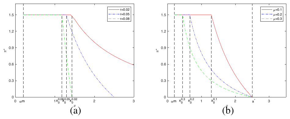
How to read it. Each curve is one strategy. To the left of its dashed vertical line the curve lies on the cap of 1.5; to the right it falls off and reaches zero at its own safe level .
What to notice. (a) The higher the risk-free rate, the lower the threshold and the closer : at the safe level is 1.43, at it equals 10 and is off the figure. (b) The higher the expected return, the smaller the share and the lower the threshold: at borrowing is needed only below 0.44.
Check, our calculation. At and the correct formula gives a share of 0.58; the figure shows about 0.6. The formula printed in section 4 would give the cap of 1.5. The threshold from (3.8) equals 1.18, 1.29 and 1.43 for the three rates, and all three vertical lines stand at these places, between 1 and 2.
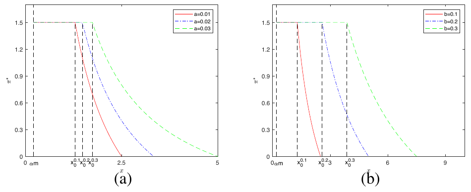
What to notice. The larger the consumption, the higher the safe level and the higher the threshold below which borrowing happens. At the safe level is 7.5 and the threshold is . The formula for from section 4 would give 6.56, while the vertical line in the figure stands at 3.9.
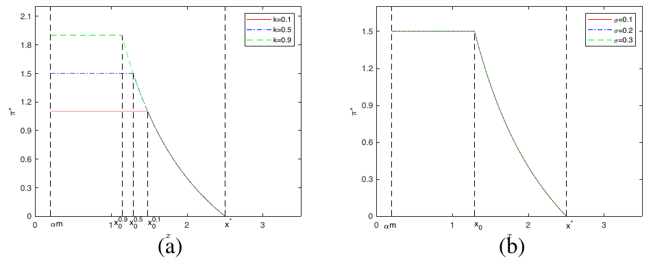
What to notice. (a) The borrowing cap changes only the flat part: 1.1, 1.5 and 1.9. The falling part of the curve is common to all three. (b) The three curves for the three volatilities lie exactly on top of one another.
The practical takeaway. As long as the constraint does not hit the cap, position size is set by the distance to the target and the ratio of the drifts, not by volatility. This is a property of the model with one asset and continuous trading; with several assets, as the authors write, it does not hold.
The probabilities the paper does not give
Since the probability formulas in the paper are printed with an error (section 6), we computed the probabilities ourselves with the corrected formula and checked them by simulating the wealth equation itself under the optimal strategy. The fixed-barrier case: , barrier , all other parameters at base values. Our calculation.
| Starting wealth | Probability of reaching 2.5 before 0.5, formula | Monte Carlo, 20,000 paths |
|---|---|---|
| 0.8 | 0.2473 | 0.2329–0.2519 |
| 1.29 () | 0.7986 | 0.7630–0.8017 |
| 1.8 | 0.9789 | 0.9537–0.9790 |
| 2.2 | 0.9994 | 0.9935–0.9994 |
The Monte Carlo range runs from the share of paths that reached the target to the share of “reached plus unresolved after 100 years”. Wealth approaches the safe level asymptotically, so some paths formally never finish; the formula lies inside the range at all four points.
5. What the paper adds to earlier work
The authors name three contributions: several risky assets instead of one (the truncation method from their own earlier paper [21] does not work here, hence the auxiliary market); a barrier that trails the maximum instead of standing still; and a numerical analysis of how the parameters matter. Problems of minimizing the probability of ruin or of drawdown come out as special cases.
6. What is shaky in the paper
What the authors concede or leave unproved
The proofs of Lemma 2.1 and of verification Theorem 3.1 are omitted with references to other authors' work ("we omit it here", "thus we omit the proof here"). For Theorem 3.2 only one of the two subcases is proved; the second “is proved similarly”. The statement that “optimality can easily be verified” after (3.6) is not verified in the text.
What the cross-check found
Probability formula (3.10) is printed with a wrong factor, and the probability it gives is zero. This is the headline result: the abstract promises "The explicit expressions for the optimal investment strategy and the maximum goal-reaching probability before drawdown are derived in closed-form."
Check of (3.10), p. 8875. Verdict: source defect.
| As printed in the source | (and similarly ), p. 8875 |
| Notation | [text, (3.7)]; is the probability [text, Theorem 3.2] |
| Assumptions | all from the text: one risky asset, , the parameters of section 4 |
| Derivation | from (3.7) , hence , with no factor [step reconstructed by us] |
| Numerically | Our script. Below the function , and with the factor the derivative grows toward (0.11 → 5·10⁵), that is, the function is convex, whereas Theorem 3.1(i) requires a concave one. The integral in the denominator diverges, and at every point. The corrected version gives 0.247 / 0.799 / 0.979 / 0.9994 and falls within the Monte Carlo range at all four points |
| Alternative reading | that in (3.10) means a different quantity than in (3.7). Ruled out: (3.10) refers directly to and from (3.9) and (3.7) respectively, and in the proof of Theorem 3.3 the same factor is carried into the derivative , so this is not a typesetting slip but an expression the authors actually worked with |
| Other places | the functions , of Theorem 3.3 contain the same factor and inherit the error |
Formula (3.9) for the region with borrowing at the cap does not satisfy the paper's own equation.
Check of (3.9), p. 8875. Verdict: source defect.
| As printed in the source | , , p. 8875 |
| How it was checked | our script: a market of two assets (our example); for each the maximum over fractions with was found by direct search, and the residual of the HJB equation was computed for the printed and for the root from our symbolic derivation (sympy) |
| Result | the printed formula gives a residual of +0.036…+0.106 and, at the boundary , a value of −8.06, whereas continuity with (3.7) requires −0.336 there. Our root gives a residual of the order of , matches the direct numerical solution to the fourth digit and equals −0.336 at the boundary |
| Alternative reading | that (3.9) is written for the auxiliary market and does not have to solve the original equation. Ruled out: by Lemma 2.1 the values coincide, and Theorem 3.1 requires to be twice smooth, that is, to be continuous at |
| In addition | with one asset the denominator is identically zero (equality in the Cauchy–Schwarz inequality), and (3.9) is undefined. The paper's numerical section is entirely on one asset; there this region reduces to , and the figures do not depend on (3.9) |
The strategy formula in section 4 has lost the division by . The text has and the threshold . From (3.11) and (3.7) with one asset it follows that the share is , and the threshold coincides with from (3.8). The figures are drawn from the correct version: at the vertical line stands at 3.87 (), not at 6.56 (); at the formula for gives an outright negative threshold of −0.31. At the printed formula gives a share of 0.80 instead of the correct 0.40.
A minor point. Section 2.1 says "we set x > m to allow the wealth process to have a financial past", although is the maximum, and by the definition of the region it should be . A typo; it does not affect the results.
What this means for trust
The strategy, that is, the main practical result, is correct: it can be derived anew from the paper's equation and matches all six panels of the figures. The probability formulas, the second half of what the abstract claims, are printed in such a way that not a single number can be computed from them. Peer review let these errors through. Not a single probability is computed or plotted in the paper, so the error could not have been spotted from its own examples.
7. What follows in practice
If wealth melts away without trading, take more risk closer to the barrier, not less. This is the model's main conclusion, and it is correct. It contradicts the familiar intuition “cut size in a drawdown”, and the contradiction is explained by the goal: that intuition is about survival over an infinite horizon, while here the task is to reach a level before a barrier in an unfavorable game. In a prop evaluation, a participant with negative drift after costs is in exactly this kind of game. The paper by Hall (2026) shows on firms' rules that even with zero edge, increasing size raises the pass probability from 0.10 to 0.43; there this works through daily observation and the trailing barrier, and negative drift adds this paper's mechanism to them.
The drawdown level does not affect the strategy, only the odds. Whether the barrier trails or stands still, whatever fraction of the maximum it is set at, the optimal share depends only on current wealth. For rules with different limit sizes this means that what changes is the answer to “is it worth buying”, not to “how to trade”. In the model. On discrete days with a contract price this has to be checked separately.
With zero drift, size does not matter at all if the barrier is fixed. This is not from the paper but our corollary from the same mathematics: with zero drift wealth is a martingale, and the probability of reaching the target before a fixed barrier equals the ratio of distances, , where is the distance to the barrier and the distance to the target, under any strategy. Size starts to matter only through the sign of the drift (costs sit inside it), through the discreteness of observation (the daily close jumps over the barrier) and through a trailing barrier. These are exactly the three mechanisms examined in the papers by Villahermosa (2026) and Hall (2026).
The probability formulas from the paper must not be used. Only (3.11) for the strategy and (3.8) for the threshold; compute the probability with the corrected formula (section 6) or by simulation.
8. Testable ideas
| No. | Idea | Type | Where to compute |
|---|---|---|---|
| 1 | Position size at the evaluation stage as a function of the distance to the target: maximum at the limit, falling toward the target as ; compare the pass probability against a constant size in a simulation of the rules | design change | Python |
| 2 | Check the sign: with positive drift after costs, the same strategy should lose to a constant small size; find the drift at which the optimum switches | diagnostic | Python |
| 3 | Check the independence of the optimal size from the limit size () on discrete daily data: in the model size does not depend on the limit, but on the daily close, where the barrier gets jumped over, a dependence may appear | audit | Python |
| 4 | Do not take the probability formulas (3.10) and Theorem 3.3 from this paper; compute the probability with the corrected formula or by simulation, and check one against the other | audit | Python |
| 5 | Measure the contribution of each of the three mechanisms through which size affects the pass probability: the sign of the drift after costs, discreteness of observation, trailing barrier; with zero drift, a fixed barrier and continuous observation the contribution of size should be zero | diagnostic | Python |