How to read this walk-through. The formulas are taken apart from scratch: in words, symbol by symbol, on numbers. The main conclusion can be taken away without reading a single formula: it is in the section “The method in one line” and in the first paragraph of section 7.
The main thesis
The Kelly criterion gives the fastest growth of wealth in the long run, but along the way wealth sinks deep, and this has long been known. The usual remedy is to bet not full Kelly but a fraction of it, “half Kelly” or “quarter Kelly”. The authors call this an “ad hoc” device: the fraction is chosen by eye, and it guarantees no specific drawdown probability.
The paper states the problem directly: maximize growth subject to the probability of ever dropping below a given fraction of starting wealth not exceeding a given number. In its original form the problem is hard, and the authors do not hide it ("seems very difficult to solve"). So they derive a sufficient condition that is easy to check and that turns the problem into a convex one, that is, one solvable by standard software. The condition is conservative: the true drawdown probability comes out lower than promised, by about a third in their examples.
For trading with a loss limit this is a direct answer to the question “what risk per trade should I take so that the chance of hitting the limit is no more than 20 %”.
1. How the problem is set up
There are bets. The fraction of wealth placed on bet is denoted ; all fractions are nonnegative and sum to one. The last bet is special: it always returns exactly 1, that is, it is the money kept in hand. Each round wealth is multiplied by , the weighted sum of returns. Rounds are independent and identically distributed.
What is. The wealth multiplier for one round. If 20 % of wealth is placed on a bet returning 1.5, another 10 % on a bet returning 0, and 70 % sits in cash, the multiplier is : wealth is unchanged.
The logarithm of wealth after rounds is the sum of the logarithms of the multipliers, that is, a random walk. Its mean step is called the growth rate. The Kelly criterion chooses the fractions so that this rate is as large as possible. The problem is convex, and for two outcomes it has the formula everyone knows: bet of wealth, where is the probability of winning and is how many times a win multiplies the stake.
In this paper drawdown is measured from starting wealth
This is the first thing to keep in mind when carrying the result over to trading. The authors define
the lowest value of wealth over all time, with starting wealth equal to 1. Drawdown is : "A drawdown of 0.3 means that our wealth dropped 30% from its initial value (one), before increasing". This is not the drawdown from the peak that backtests have made familiar. It is exactly a prop firm's static loss limit: “the account is closed if the balance falls 10 % below the starting balance”.
The horizon is infinite: the condition concerns the entire future path, not the evaluation month.
2. The method in one line
What this is. A check that can be run for any set of bets before play starts. If it holds, the probability of ever dropping below a fraction of starting wealth is strictly less than .
What each symbol means. (alpha): the wealth threshold as a fraction of starting wealth. A 10 % loss limit is . (beta): the acceptable probability of breaching this threshold even once. (lambda): the number that comes out of them. Read it as the “risk-aversion parameter”. : the average over all possible outcomes of one round. : the wealth multiplier for a round raised to the power minus lambda. This inflates bad rounds (multiplier below 1) and compresses good ones. : the natural logarithm.
Step by step. 1) Choose and . 2) Compute by dividing the logarithms. 3) For the proposed fractions, go through all outcomes of a round, raise each outcome's multiplier to the power and average with the probabilities as weights. 4) If the result is no greater than one, the fractions pass.
A worked example on the paper's numbers. , : “a drawdown greater than 30 % with probability no higher than 10 %”. Then . The paper notes that the same check also promises : losing half of wealth can happen in no more than 1.1 % of cases.
Why this matters. A single number sets the whole risk curve at once: for any . Choose it for one threshold and you get guarantees for all the others.
The RCK problem (risk-constrained Kelly) is obtained by replacing the hard condition with this one:
It is convex because is convex in the fractions, and an average of convex functions is convex. For a finite number of outcomes the condition is written with the log-sum-exp function, and CVXPY solves the problem directly; the specification takes six lines in appendix B.
3. Why the bound holds
This section can be skipped: the conclusions below do not depend on it.
The proof rests on Wald's identity from random walk theory (lemma 5 in the appendix). Its meaning can be conveyed like this. Take the quantity , wealth raised to the power minus lambda. The condition means that on average this quantity does not grow from one round to the next. It starts at one. At the moment wealth first falls below , it becomes greater than , that is, greater than . A quantity that does not grow on average and starts at one can rise above with probability no greater than . Hence the bound.
The link to Hall (2026), our derivation. If the logarithm of the per-round multiplier is normally distributed with mean and spread , then at , and the bound becomes . This is exactly the first-passage formula for Brownian motion with drift that Hall gives as Proposition 3. Two papers published ten years apart, neither citing the other, use one and the same bound: one for a fraction of wealth, the other for a limit in dollars. Checked numerically: with , , both forms give 0.5905.
Two limiting regimes
For very large the condition requires the multiplier to be at least one in every outcome: only risk-free bets are allowed.
For small the condition turns into
What this is. The variance of log growth divided by mean growth must not exceed . This is the same “return to risk” relationship as in Markowitz, only for the logarithm of wealth.
Our example. At the variance of log growth per round may be no more than of the mean growth per round.
4. What the numerical examples show
A finite number of outcomes
Twenty bets (nineteen risky ones and cash), a hundred outcomes. Returns are uniform from 0.7 to 1.3, and in addition thirty randomly chosen returns were replaced with 0.2 and another thirty with 2. The authors reckon that at least one “extreme” return occurs in a round with probability about 0.45; a recount gives , which matches. Each set of bets was run over ten thousand paths of a hundred rounds.
| Bet | Growth rate | Bound | Monte Carlo risk | Bound / risk |
|---|---|---|---|---|
| Kelly | 0.062 | n/a | 0.397 | n/a |
| RCK, | 0.043 | 0.100 | 0.073 | 1.37 |
| RCK, | 0.047 | 0.141 | 0.099 | 1.42 |
Table 1 of the paper, the last column is ours. Full Kelly falls below 70 % of starting wealth in four cases out of ten. RCK with a 10 % guarantee gives 7.3 % and loses about a third of the growth rate. If is relaxed to 5.5, the risk comes right up to 10 % and growth recovers to 0.047.
From this the authors draw a careful conclusion about the hardest problem: its optimum lies between 0.047 and 0.062. The lower bound comes from the bet with : it is feasible according to Monte Carlo, although it has no formal guarantee.
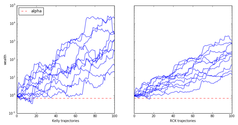
How to read it. Horizontally, the round number, from 0 to 100. Vertically, wealth on a log scale: each division is ten times the previous one. The red dashed line is at 0.7 of starting wealth.
What to notice. On the left the paths spread apart by about three orders of magnitude by the end, and four out of ten dip below the dashed line. On the right the fan is noticeably narrower, and one path goes below the line.
The practical takeaway. RCK buys a narrow fan at the price of the median outcome: by round one hundred the right-hand paths are about an order of magnitude below the left-hand ones.
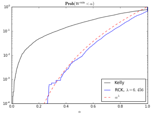
How to read it. Horizontally, the threshold , from 0 to 1. Vertically, the share of paths that fell below that threshold, on a log scale. The black curve is full Kelly, the blue one RCK, the red dashed line the promised bound .
What to notice. The blue curve lies below the red one almost everywhere and runs almost parallel to it: the bound is not just valid, it repeats the shape of the true distribution. The black curve is one to two orders of magnitude higher: under full Kelly the chance of losing 90 % of wealth is on the order of one to two percent.
What the authors do not comment on. For from 0.27 to 0.33 the blue step rises above the dashed line: about 6–9 paths out of 10,000 against roughly 2–8 that the bound allows. The bound is proven, so this is either noise on single events or a consequence of the numerical solution satisfying the condition only approximately. The text says not a word about it.
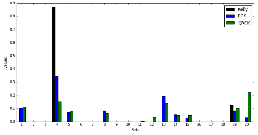
How to read it. Horizontally, the bet number from 1 to 20; the twentieth is cash. Vertically, the fraction of wealth.
What to notice. Kelly puts 87 % into one bet (number 4) and the rest into bet 19, with nothing in cash. RCK cuts bet 4 by a factor of two and a half, spreads wealth across eight risky bets and leaves a little in cash. QRCK keeps more than 20 % in cash.
The practical takeaway. The drawdown constraint works as forced diversification. It is not a separate rule; it comes out of the condition by itself.
| Bet | Growth rate | Bound | Monte Carlo risk |
|---|---|---|---|
| QRCK, | 0.054 | 1.000 | 0.218 |
| QRCK, | 0.027 | 0.100 | 0.025 |
| QRCK, | 0.044 | 0.368 | 0.100 |
Table 2 of the paper. At the same the quadratic version (section 5) grows at 0.027 against 0.043 for RCK, and its risk is 2.5 % where 10 % is allowed: it overinsures. Tuned to a 10 % risk, it grows at 0.044 against 0.047 for RCK.
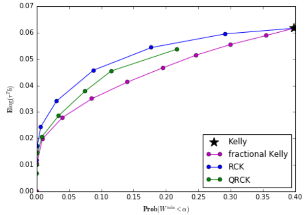
How to read it. Horizontally, the probability of dropping below 0.7 of starting wealth. Vertically, the growth rate. Each point is one bet; the curves connect bets of one family at different or different Kelly fractions. The star is full Kelly.
What to notice. The blue RCK curve lies above the purple fractional Kelly curve everywhere. At 10 % risk fractional Kelly grows at about 0.035–0.037, RCK at 0.047. The authors give 0.035.
The practical takeaway. On a distribution with extreme outcomes fractional Kelly is markedly inefficient: it cuts all bets proportionally, although the risk is created by specific ones.
A continuous distribution
A mixture of two lognormal distributions, 20 assets, a million observations for solving and ten thousand paths for checking.
| Bet | Growth rate | Bound | Monte Carlo risk | Bound / risk |
|---|---|---|---|---|
| Kelly | 0.077 | n/a | 0.569 | n/a |
| RCK, | 0.039 | 0.100 | 0.080 | 1.25 |
| RCK, | 0.043 | 0.131 | 0.101 | 1.30 |
Table 3 of the paper, the last column is ours. Here full Kelly breaches the threshold in 57 % of cases, and RCK halves growth.
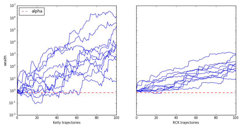
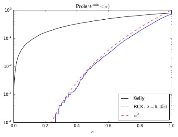
How to read figures 5 and 6. The same way as 1 and 2. In figure 6 the blue curve lies below the dashed line across the whole visible range; there is no excess like the one in figure 2.
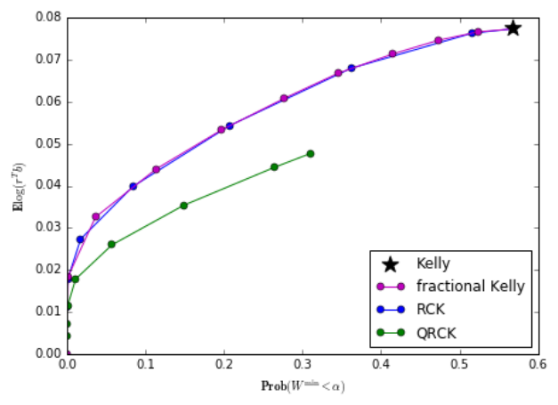
How to read it. The axes are as in figure 4.
What to notice. The blue RCK points lie on the purple fractional Kelly curve. There is no gain. The green QRCK curve is noticeably below both.
The practical takeaway. On a smooth, market-like distribution fractional Kelly is as good as RCK. The advantage of RCK appears where the distribution has extreme outcomes spread unevenly across the bets.
5. The quadratic approximation and Markowitz
If the per-round multiplier is close to one, the logarithm and the power can be replaced with the first terms of their expansions. Denoting the excess return , the authors obtain the quadratic problem QRCK:
What this is. The same RCK, but with the mean and the second moment instead of the full distribution. Any quadratic optimization software solves it.
What each symbol means. (rho): how much a bet increases wealth above one. : the mean gain per round. : the mean square of the gain, that is, the variance plus the square of the mean.
Step by step. The condition can be rewritten as “the mean gain is no less than times the mean square of the gain”. The larger , the tighter the constraint on the swing.
The authors prove that, in the absence of arbitrage, the QRCK solution is always a Markowitz portfolio for some risk-aversion coefficient. Our interpretation, not in the paper: this explains why the Markowitz approach worked “by eye” for so long on the drawdown problem, since it is itself a rough approximation of the right problem.
A simple corollary that is not in the paper, our derivation. For a single bet the QRCK condition gives a size no greater than , where is the mean gain and the mean square of the gain. Kelly in the same approximation equals . Therefore
A worked example on the paper's numbers. At this is , that is, “a little over quarter Kelly”.
A check against the exact solution, our example. A trade with a reward-to-risk ratio of 1.5 and a 42 % win rate, a 10 % loss limit (), and an acceptable 20 % chance of hitting it (). Then . Kelly risks 3.33 % of wealth per trade. The exact RCK, found by bisection on the paper's condition, risks 0.41 %, that is, 12.2 % of Kelly; the formula gives 12.3 %. Monte Carlo over 2,000 trades: full Kelly hits the limit in 88 % of cases, RCK in 18.8 % against the promised 20 %. For a 4 % limit at : , exact RCK 6.5 % of Kelly, formula 6.6 %.
6. What is shaky in the paper
What the authors admit themselves
The original problem with a true constraint on drawdown probability remains unsolved: RCK solves a stricter one, and the price of that strictness is visible in the tables (10 % promised, 7–8 % obtained). The authors call the bound "reasonably close" in the abstract and write that the Monte Carlo risk is below the bound, "but not dramatically so". Our recount from their tables: the bound exceeds the actual risk by a factor of 1.25–1.42, which agrees with their words "typically around 30% or so higher than the actual risk".
The stochastic gradient for the continuous case "can be slow to converge", and the parameters and have to be guessed and then checked. This is stated honestly.
What turned up in the cross-check
The abstract promises more than section 7.2 shows. The abstract says without qualification: "Simulations show that this method yields bets that out perform fractional-Kelly bets for the same drawdown risk level or growth rate." In section 7.2.2, on the only example with a continuous distribution, the opposite is stated: "The fractional Kelly bets, in this case, show instead the (essentially) same performance as RCK." Figure 7 confirms it: the blue points lie on the purple curve. Superiority over fractional Kelly is shown on one of the two distributions, the artificial one with extreme outcomes. A reader who stops at the abstract will come away with a stronger claim than the data support. For a market whose returns are closer to the second example, this matters.
Typos in the two-outcome problem (10). The second term of the objective is missing a logarithm: it reads instead of . Further down, in the equation for the bisection, the exponent is written as instead of . Both typos were checked against the rendered page 9; they are not a text-extraction artifact. They do not affect the conclusions, but the formula from (10) cannot be copied into code as is.
A minor point. In section 7.1.1 the “Kelly problem with drawdown risk” is twice cited with a reference to (9), although it is problem (5); (9) is only the condition itself.
What the paper does not cover
Drawdown is measured from starting wealth, the horizon is infinite, rounds are independent. For trading these are three separate assumptions, and each one matters. The paper does not model a limit trailing the balance high at all (section 7). The model has no dependence between days, no losing streaks and no changes in volatility. The examples are synthetic; none of them uses market data.
7. What follows in practice
For a static loss limit, position size is chosen by formula, not by eye. Compute from the limit and the acceptable chance of hitting it, then find the largest size at which the average of over the distribution of trades is no greater than one. For a single trade this is a one-dimensional bisection; a quick estimate is of Kelly (section 5). With a 10 % limit and a 20 % chance of hitting it, that is about one eighth of Kelly. This is noticeably less than what is usually risked on prop accounts.
The bound does not apply to a trailing limit. If the limit is measured from the balance high and the horizon is unlimited, any strategy that can have losing rounds will sooner or later hit it with probability one: drawdown from the peak is reset with every new high. A meaningful question for a trailing limit can only be posed on a finite horizon, and that is the subject of Yuan & Li (2021) and Hall (2026). This is our derivation; it is not in the paper.
RCK maximizes growth, not the probability of passing an evaluation. These are different problems. At the evaluation stage, where what matters is reaching the target before the limit, the criterion is different, and there, with zero or negative edge, it pays to increase size (Hall, 2026, section 5.3; Yuan & Li, 2021). RCK answers the funded-account question: how to grow without losing the account.
Fractional Kelly is no worse than RCK on smooth distributions and loses on fat-tailed ones. For a portfolio of many strategies with rare large losses, RCK with historical days as finite outcomes can give a noticeably better trade-off than proportional scaling down. This can be checked on your own history: the portfolio's historical days are exactly the “finite number of outcomes” from section 4.
8. Testable ideas
| No. | Idea | Type | Where to compute |
|---|---|---|---|
| 1 | Risk per trade for a static loss limit via RCK: , the largest fraction with over the strategy's distribution of trades in R-multiples; compare with the quick estimate of of Kelly | diagnostic | Python |
| 2 | Bootstrap real trades to measure how many times the bound exceeds the actual breach frequency; the paper has 1.25–1.42 on synthetic data, market tails may behave differently | acceptance metric | Python |
| 3 | Do not apply the RCK bound to a limit trailing the peak: with an infinite horizon the probability of hitting it equals one; for a trailing limit compute only over the evaluation horizon | audit | any |
| 4 | Portfolio RCK for a set of strategies: historical days as finite outcomes, CVXPY with log-sum-exp, the constraint “portfolio stays at or above 0.9 of starting value with probability ≥ 0.8”; compare with weights from drawdown correlation or with equal weights | design change | Python |
| 5 | Plot the “growth rate versus breach probability” curve for RCK and for fractional Kelly on your own history (the analog of fig. 4 and 7); test the paper's hypothesis that RCK gains only when tails are uneven | acceptance metric | Python |
| 6 | Use the quadratic version QRCK (Markowitz with a tuned ) only as a starting point: in the paper at the same risk it gives growth of 0.044 against 0.047, and at the same it gives 2.5 % risk instead of the allowed 10 % | diagnostic | Python |
| 7 | Check that the numerical RCK solution satisfies on an independent sample, not on the one it was solved on; in figure 2 of the paper the sample risk is above the bound in places | audit | Python |