How to read this walk-through. The essentials are in two places: the section “The method in one line” (the whole recipe; you can take it and skip the rest) and section 9 (out-of-sample results for 1964–2014). Sections 3–5 take the formulas apart symbol by symbol; if you do not need the formulas, you can skip them. Section 7 is for those who want to understand how the parameters were chosen and how much the result depends on that choice. The numbers come from the paper's tables and text, we did not recompute them; examples marked “our example” were made up by us for illustration.
The main thesis
There is a well-known argument against Markowitz portfolio theory (DeMiguel and co-authors): the equal-weight portfolio compares favorably with optimized ones. The theory is usually applied with parameters estimated from long-term returns. The authors argue that the issue is the horizon. If all three quantities are estimated over the last year and the portfolio is rebuilt every month, that is, if one relies on the persistence of return, volatility and correlation rather than on their long-term averages, the result beats equal weight. The authors call this persistence of the three quantities generalized momentum: "we assume persistence in the short-term, not only for R, but also for V and C" (abstract).
The model itself is simple. Every month a score is computed for each asset: return raised to one power, multiplied by “one minus the correlation with the index” raised to another power, and divided by volatility raised to a third. The authors call the exponents elasticities, hence the name Elastic Asset Allocation. An asset's weight is proportional to its score; only a few of the best are taken; assets with non-positive return get zero, and their share by count goes to the safe asset.
To avoid fitting the parameters to the same data they are tested on, the authors split a century of monthly data in half. Everything is chosen on 1914–1964 and tested on 1964–2014. On three universes of indices (7, 15 and 38 asset classes) both final versions deliver, out-of-sample, a higher return than the equal-weight portfolio of the same assets, and a maximum drawdown of 8.6 to 25.3 % against 34.8–43.4 % for equal weight.
1. Where EAA came from
The paper continues two earlier models by Keller. FAA (Flexible Asset Allocation, 2012) ranks assets on three attributes: return (R), volatility (V) and correlation with the equal-weight index (C). The ranks are added up with weights, and the assets with the best total rank go into the portfolio in equal shares. MAA (Modern Asset Allocation, 2013–2014) does the same in the spirit of Markowitz: it uses Elton's single-index model (1976), in which an asset's return is split into a part explained by the market and an asset-specific part, and it obtains an analytical formula for the long-only portfolio that is optimal by Sharpe.
Both models shared a weakness that the authors name directly: "Testing for FAA and MAA was conducted using daily data", and daily data for most indices exist only for recent decades. Those decades fell almost entirely into one regime: rates and inflation kept falling. The new paper moves to monthly data over a hundred years in order to capture eras of rising and falling rates, inflation and economic growth.
EAA differs from FAA in one step. Instead of ordinal ranks (first, second, third), the attribute values themselves are taken and multiplied together, each raised to a power. A rank loses the information about how much better an asset is than its neighbor; the product keeps it. And an asset's weight becomes proportional to its score, rather than equal for all selected assets as in FAA.
What correlation with the equal-weight index is. The index here is not the S&P 500 but a portfolio of all assets of the universe in equal parts, rebuilt every month. An asset's correlation with it shows how much the asset moves together with the “typical” asset of the universe. Bonds in a universe dominated by stocks usually have a low correlation with such an index, so the EAA formula rewards them. What is rewarded is not low volatility as such but the asset's ability to move differently from the rest.
2. The method in one line
Once a month: for each asset compute the average excess return over 1, 3, 6 and 12 months and the correlation of its monthly returns over 12 months with the equal-weight index; give the assets with positive return a score by the “golden” formula; take the few best and allocate capital in proportion to the score; give a share of the portfolio equal to the share of assets with non-positive return in the whole universe to 10-year US Treasuries.
The recipe from section 4.6 of the paper:
- : the asset's average total excess return over the last 1, 3, 6 and 12 months (the authors dropped 9 months because that horizon did not help on the training period). Excess means above the yield of 13-week Treasury bills.
- : the standard deviation of the last 12 monthly returns, nominal, without subtracting the rate.
- : the correlation of the asset's last 12 monthly nominal returns with the index.
- The index: the equal-weight () monthly nominal return of all assets of the universe.
- The score by formula (4) with the chosen elasticities; when the score and the weight are zero.
- The portfolio holds the assets with the best positive score, weights proportional to the scores.
- Crash protection: a share , equal to the share of assets in the whole universe with non-positive excess return, goes to the safe asset (10-year US Treasuries).
- Rebalancing at the end of each month, costs of 0.1 % one-way, no leverage.
The two final “golden” score formulas:
What this is. The asset score in the two final models. Both use only return and correlation, with no volatility (section 3 explains why). Both formulas follow from the paper's general formula (4) by substituting the chosen exponents: the defensive one at and , the offensive one at and .
What each symbol means. (“z i”): the score of asset number . (“r i”): its average excess return over 1, 3, 6 and 12 months. (“c i”): its correlation with the equal-weight index over 12 months, from −1 to 1. : the square root.
Step by step. For each asset with positive : subtract the correlation from one and multiply by the return. In the defensive model take the square root of this product. In the offensive model multiply the result by the return once more (that is, return squared). Then select the best and divide each score by the sum of the selected scores: these are the shares.
Our example. Two assets. A has a return of 2 % and a correlation with the index of 0.8; B has a return of 1 % and a correlation of 0.2. Defensive model: , ; shares of about 41 % and 59 %, so the less profitable but less market-linked B gets more. Offensive model: , ; equal shares. Squaring the return in the offensive model offsets B's advantage on correlation.
Why this matters. The two formulas set two extremes of one idea. The defensive one gently blends return and diversification and gives weights closer to equal. The offensive one pulls capital harder toward the return leader.
3. The main formula and its parts
Formula (1) of the paper, from the rendered page 3:
What this is. The generalized momentum score of an asset. The asset's weight in the portfolio is proportional to it.
What each symbol means. (“w i”): the share of asset in the portfolio. : “proportional to”, that is, equal up to a common multiplier, which is then chosen so that the shares add up to one. : the score. , , : return, volatility and correlation with the index. , , (“w R”, “w V”, “w C”): nonnegative exponents on return, volatility and “one minus correlation”; these are the elasticities.
Step by step. Raise the return to the power , the expression to the power , multiply them, and divide by volatility raised to the power . The higher the return and the lower the volatility and correlation, the higher the score.
Why this matters. One formula instead of three ranks. By changing three numbers you can get equal weights, risk parity, or a pull toward the return leader (section 5).
The shares are normalized by the long-only condition, formula (2):
Why correlation enters as rather than on its own. The authors point out that after the filter and the replacement of with , all three factors are nonnegative by construction, and "the fractional exponent of a negative value is undefined". A negative number raised to a fractional power is undefined, so without these two measures the formula would not work.
Why the exponents are called elasticities. In economics an elasticity is a ratio of relative changes: by how many percent one quantity changes when another changes by one percent. The authors' example: an elasticity means that when rises by 10 %, the weight changes by about 5 %. Our refinement: the elasticity describes the change in the score exactly; the share after normalization changes a little less, and the larger the asset's share in the portfolio, the smaller the change, because the normalizing denominator grows along with it.
The scaling exponent
For the computations the authors rewrite formula (1) in an equivalent form, formula (4):
What this is. The same score, but the exponent on return is fixed at one, and the whole expression is raised to a common power . The elasticities and are now relative to return.
What each symbol means. (“w S”): the scaling elasticity, which controls how concentrated the portfolio is in the leaders. The other symbols are the same as in formula (1).
Step by step. Compute the expression in parentheses and raise it to the power . At any positive number raised to the zero power equals one, all selected assets get the same score, and the portfolio becomes equal-weight. At a very large the gap between the best asset and the rest becomes enormous, and almost all the capital (except the protective share) goes to one asset.
A worked example on the paper's numbers. So that the best can still be selected at , the authors add to a tiny number, : the scores are almost equal, the weights practically the same, but the order of the assets is preserved. This variant essentially repeats FAA with equal shares.
Why this matters. One knob instead of two decisions. sets how much to reward diversification (the authors call it hedging), sets the concentration.
One more property the authors note: the formula does not depend on the units of return and volatility. Monthly or annual, percent or fractions, the common multiplier drops out in normalization. This does not hold for correlation: it is unit-free and bounded between −1 and 1, so the shift by one in makes sense.
Why volatility is switched off
In section 4.7 the authors write that on the training period the volatility term "had little impact on strategy performance" given and . They give the explanation with a hedge: "This is probably related to the fact that ci and vi are collinear", meaning that most bonds have both low volatility and low correlation with the index, and the two attributes say the same thing. For simplicity is set in all tests. Two tunable exponents remain, and .
4. Selecting the best and crash protection
How many assets to take
As in FAA, only the top part of the universe by score goes into the portfolio. At first the authors set it as a fraction of , rounded down; on the training period it turned out that the best fraction decreases as grows. To avoid adding one more search dimension, the number of assets is set as a function of the square root of (footnote 4 of the paper):
What this is. How many of the best assets to hold in the portfolio for a universe of assets.
What each symbol means. : rounding up to an integer. : rounding down. : the smaller of two numbers. : the square root of the number of assets.
A worked example on the paper's numbers. : the square root is about 2.65, rounded up 3, plus one 4; half is 3.5, rounded down 3; the smaller of 4 and 3 is 3. The authors give the result for all three universes: 3 assets at , 5 at , 8 at .
Why this matters. In a small universe hold half; in a large one noticeably less than half. When the composition of the universe changes over time (in the large universe some indices appear only by the 1970s, and by 2014 there are fewer of them again), the number selected changes along with it.
Crash Protection
The protection is built on absolute momentum: an asset with non-positive excess return is considered falling. The share of the portfolio given to the safe asset equals the share of such assets in the whole universe, not among the selected ones. Formula (3):
What this is. How much capital remains for the selected assets after the protective allocation.
What each symbol means. (“w CP”, from crash protection): the share of assets in the whole universe with . The sum on the left runs over the selected assets.
A worked example on the paper's numbers. The universe has 11 assets, , and 7 of the 11 have non-positive return. Then , that is, 64 % of the portfolio goes to the safe asset. The remaining 36 % is split in proportion to the scores among four assets: the half rule would allow five, but only four have a positive return.
Why this matters. The protection switches on gradually. When one asset in ten falls, 10 % goes to protection; when almost the whole market falls, almost the whole portfolio does. There is no abrupt all-or-nothing switch.
Which asset is the safe one was also chosen on the training period. The candidates were three-month Treasury bills and US bonds of various kinds (10 and 30 years, municipal, corporate). In the authors' words, "US Gov10y was a clear winner" on all universes, and in all tests the safe asset is 10-year US government bonds.
5. Special cases: what the formula can do
Section 3 and appendix A of the paper show that well-known allocation schemes follow from the EAA formula by substituting exponents. This is the authors' argument for the chosen form of the formula.
| Exponents in formula (1) | Asset weight | What scheme this is |
|---|---|---|
| (or in formula 4) | equal weights | |
| , the rest 0 | naive risk parity | |
| , the rest 0 | minimum variance with zero market volatility | |
| , , | return momentum adjusted for variance | |
| , , | an approximation of maximum diversification |
How to read it. Each row is one of the paper's formulas (5)–(9). “Naive” risk parity means that correlations between assets are ignored: the weight is inversely proportional to volatility, and each asset contributes roughly the same risk of its own. The rule of selecting the best and crash protection, in the authors' words, can be applied on top of any of these schemes.
The authors derive the link to Markowitz theory through the MAA model. In the single-index model the long-only portfolio that is optimal by Sharpe has an analytical formula (A.1):
What this is. An asset's weight in the optimal portfolio when the returns of all assets are linked to each other only through a common market index.
What each symbol means. (“t i”): the Treynor ratio, the asset's return per unit of its beta. (“b i”): the asset's beta to the index, where is the volatility of the index. (“s i”): the asset's own (idiosyncratic) variance, the part of its fluctuations the index does not explain. : the Treynor threshold; assets with below the threshold get zero.
Step by step. Find the beta and the own variance of each asset, compute the Treynor ratio, drop the assets below the threshold, and give the rest a weight proportional to return per unit of own variance, adjusted for the distance from the threshold.
Why this matters. This is the benchmark that EAA approximates. The threshold is complicated to compute (the authors refer to the appendix of their 2014 paper), and in EAA it is replaced by the simple rule “take the best”.
If the Sharpe ratios of all assets are assumed equal, MAA yields a maximum diversification variant, which the authors approximate with a Taylor series, formula (A.2):
What this is. The approximate weight in the maximum diversification portfolio.
What each symbol means. : the correlation threshold; assets whose correlation with the index is above the threshold get zero. : the power to which is raised.
A worked example on the paper's numbers. With a threshold the approximation, in the authors' words, is near perfect for correlations around zero and good for from −0.3 to 0.8. The exponent on is then .
Why this matters. Here one recognizes the term of the EAA formula with and volatility to the first power. Hence the authors' argument: the correlation factor in EAA is not an arbitrary add-on but a simplified form of the optimal portfolio when the market has a common component.
The appendix's conclusion in the authors' words: EAA exactly reproduces the MAA variants without a common market component and approximates the variants with one well through the term .
6. Data, split and metric
Period and split. Monthly data from April 1914 to August 2014. The training period (IS, in-sample) runs from the end of April 1914 to March 1964, the test period (OS, out-of-sample) from April 1964 to August 2014. The authors explain why they train on the first half rather than the second: recent decades were a "dominant bond regime" with almost continuously falling rates, while 1914–1964 is more varied: high and low, rising and falling rates, and the heaviest stock market crash of the century.
Three universes. All series are monthly total return indices with reinvested dividends, from MSCI, Fama/French, Ibbotson, Barclays and Global Financial Data, extended in recent years with the closest analog indices and ETFs from Yahoo and Bloomberg.
| Universe | Composition | How many assets in practice |
|---|---|---|
| , small global | S&P 500, EAFE, emerging markets, US technology, Japan's Topix, 10-year US Treasuries, US high-yield bonds | most of the data from 1913 |
| , US sectors | 10 Fama/French sectors and five kinds of US bonds | from 2 assets in 1914 to 15 from 1927 to 1964 |
| , large global | all of the above plus small caps, GSCI, gold, foreign bonds, TIPS, REITs, five FTSE indices, Japanese 10-year bonds, three Dow indices, currency, timber | from 4 in 1914 to 28 in 1964; all 38 only from 1994 to mid-2011, 13 by 2014 |
The 7- and 15-asset universes were chosen from the large one so as to have as long a history as possible.
A 12-month window. Volatility and correlation are computed from 12 monthly observations. The authors admit that this is little compared with daily data (about 21 observations a month), but they write that there is a trade-off between data density and the aging of information, and that by their tests 12 observations are enough.
Why drawdown rather than volatility. The authors accept the Sharpe ratio as a legitimate optimization target, but over a horizon of decades they care more about heavy tails: 1929 and 2008. So risk is measured by the maximum drawdown . The authors' argument: after a 40 % fall, like the S&P 500 in 2008, a 66 % gain is needed to get back to the previous peak, and the market's average annual return is only a small fraction of that. And a caveat right away: "D does not stabilize over time, as V does", the probability of a large drawdown grows with the length of the period.
The optimization metric, formula (10), is the Calmar ratio with a threshold:
What this is. How much annual return above the threshold there is per unit of maximum drawdown.
What each symbol means. : the compound annual growth rate of capital (CAGR) after costs. : the return threshold. : the maximum drawdown over the whole period. and : the same metric with a threshold of 5 % and 10 % a year.
A worked example on the paper's numbers. The defensive model on the 7-asset universe out-of-sample: , , the table gives , that is, each percent of drawdown comes with 0.424 percent of annual return above 5 %.
Why this matters. The 5 % threshold, in the authors' words, is close to the preferences of an investor with average risk aversion (a coefficient of 3, after Ang, 2012). A more aggressive investor fits a 10 % threshold. was chosen as the main metric.
How to read the numbers in the paper's tables. All metrics in the tables are written in percent, including Sharpe and Calmar. A Sharpe of 126.6 % is a ratio of 1.266, a Calmar of 70.8 % is 0.708. , , : Sharpe with a threshold of 2, 5 and 10 % instead of the risk-free rate; on the training period the bill rate is about 2 %, so there is the ordinary Sharpe. “3y” (in the tables “3y>EW” or “3y (Roll >=EW)”): the share of rolling three-year periods in which the model beat the equal-weight portfolio of all assets of the universe on return. The comparison is always with this equal-weight portfolio, rebuilt monthly, and additionally with the S&P 500.
7. The 1914–1964 search: 49 scenarios
Both exponents were searched over seven values: 0, 25, 50, 75, 100, 150 and 200 %. In total combinations per universe.
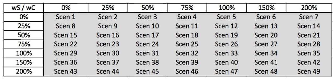
How to read it. The row sets (concentration), the column (the reward for low correlation). The scenario number is the cell number, and further on the results tables refer to scenarios only by number. For example, scenario 19 is , ; scenario 45 is , ; scenario 7 is , .
What to notice. The top left corner is equal weights without regard to correlation; the bottom right is the most concentrated portfolio with the strongest reward for diversification.
The authors plot each of the 49 backtests as a point on a plane with drawdown on the horizontal axis and return on the vertical. This is the Calmar scatter, an analog of the familiar risk-return diagram in which maximum drawdown takes the place of volatility.
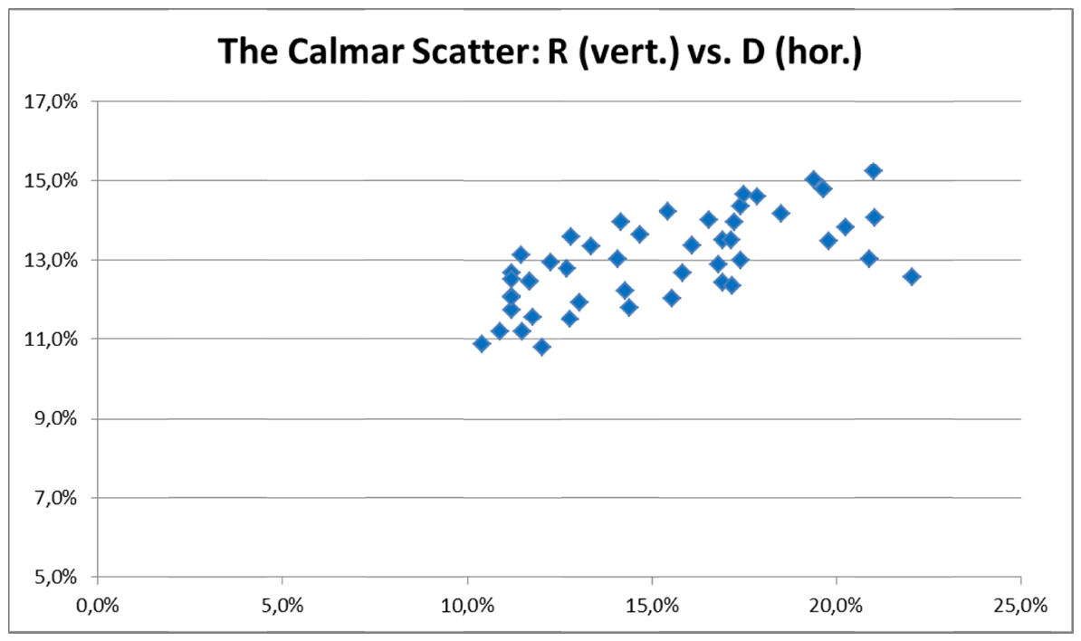
How to read it. Each point is one of the 49 scenarios on the 7-asset universe. Horizontally, the maximum drawdown over 1914–1964; vertically, the average annual return.
What to notice. All 49 variants, by eye from the figure, lie in a narrow band: drawdown roughly from 10 to 22 %, return roughly from 11 to 15 %. For comparison, the equal-weight portfolio of the same assets over this period had a drawdown of 54.9 % with a return of 8.9 %, the S&P 500 83.5 % with 10.1 %. Almost any values of the two exponents on this universe give a result far better than equal weight; the main work is done by the selection, the protection and the formula itself, not by fine-tuning.
The points for which there is no more profitable variant at a given drawdown and no variant with a smaller drawdown at a given return form the upper left envelope. The authors call it the Calmar frontier, by analogy with the Markowitz efficient frontier.
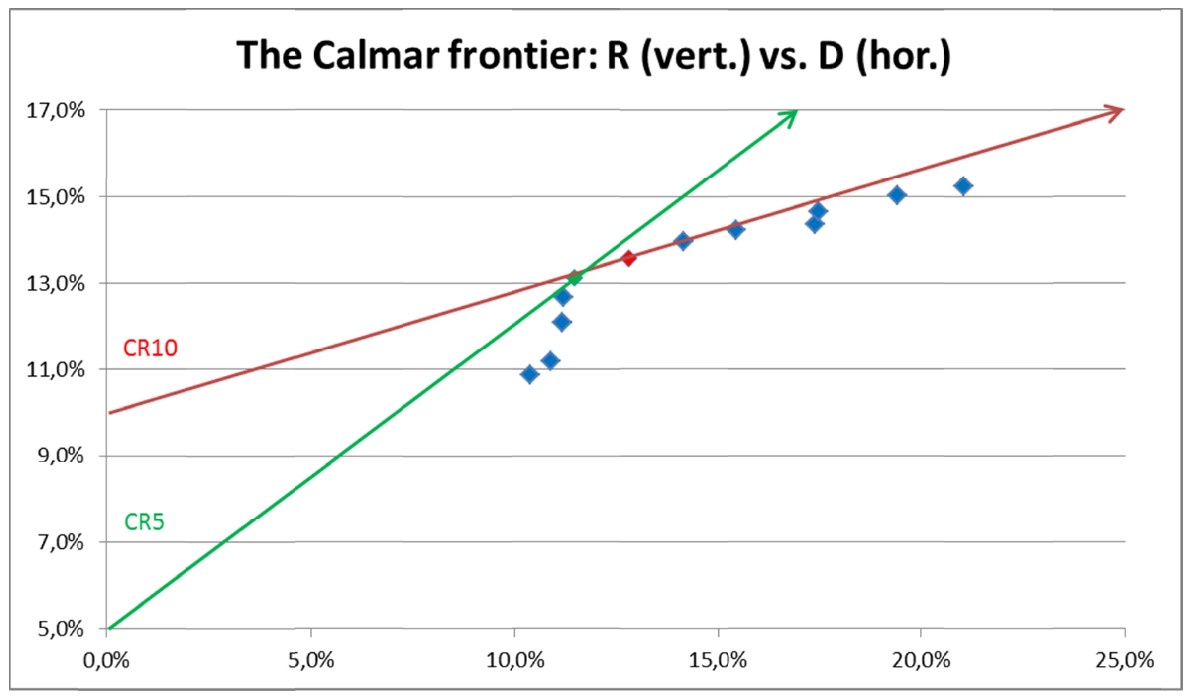
How to read it. The blue points are the 12 scenarios out of 49 that lie on the frontier. The green line starts at 5 % on the vertical axis: the point where it touches the frontier tangentially has the best . The red line starts at 10 % and touches the frontier at the point with the best (the red point).
What to notice. The higher the threshold, the flatter the line and the further right the point of tangency: at a 10 % threshold it pays to accept more drawdown for the sake of return. Hence two candidates, a defensive one and an offensive one.
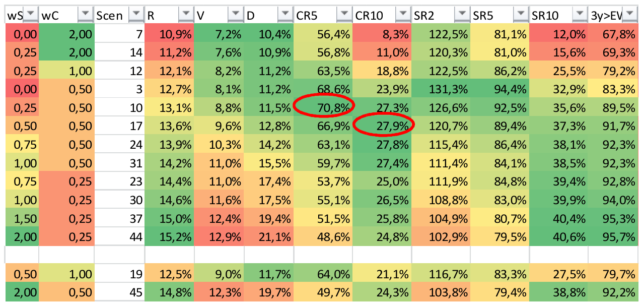
How to read it. The twelve rows at the top are the frontier scenarios, from the most defensive (scenario 7, drawdown 10.4 %) to the most offensive (scenario 44, return 15.2 %). Below the empty row are the two “golden” scenarios discussed in section 8. With red ovals the authors circled the best (70.8 %, scenario 10) and the best (27.9 %, scenario 17).
What to notice. From top to bottom broadly falls (from 2 to 0.25), while does not rise monotonically: at scenario 3 it is back to zero. Return and drawdown rise together. There is not a single scenario with on the frontier; the authors conclude from this that the reward for low correlation works. The share of three-year periods in which the model beat equal weight rises from 67.8 % for the most defensive to 95.7 % for the most offensive.
On the training period the picture across the three universes is as follows:
| Universe, IS | Best by CR5 | Best by CR10 | Most defensive | Most offensive |
|---|---|---|---|---|
| sc. 10 ( 25 %, 50 %): R 13.1 %, D 11.5 % | sc. 17 (50 %, 50 %): R 13.6 %, D 12.8 % | sc. 7: R 10.9 %, D 10.4 % | sc. 44: R 15.2 %, D 21.1 % | |
| sc. 20 (50 %, 150 %): R 8.6 %, D 12.5 % | sc. 43 (200 %, 0): R 11.2 %, D 39.1 % | sc. 35: R 7.6 %, D 11.6 % | sc. 43 | |
| sc. 19 (50 %, 100 %): R 11.5 %, D 10.9 % | sc. 45 (200 %, 50 %): R 14.0 %, D 21.9 % | sc. 7: R 8.3 %, D 9.1 % | sc. 44: R 14.2 %, D 30.9 % |
And the comparison of the best variants with the equal-weight portfolio over the same period:
| Universe, IS | Model | R | V | D | CR5 | Sharpe | 3y |
|---|---|---|---|---|---|---|---|
| sc. 10 / sc. 17 | 13.1 / 13.6 % | 8.8 / 9.6 % | 11.5 / 12.8 % | 70.8 / 66.9 % | 1.27 / 1.21 | 89.5 / 91.7 % | |
| equal weight | 8.9 % | 10.1 % | 54.9 % | 7.1 % | 0.68 | ||
| sc. 20 / sc. 43 | 8.6 / 11.2 % | 7.1 / 12.2 % | 12.5 / 39.1 % | 29.0 / 15.8 % | 0.93 / 0.75 | 37.7 / 62.3 % | |
| equal weight | 8.0 % | 13.6 % | 67.6 % | 4.4 % | 0.44 | ||
| sc. 19 / sc. 45 | 11.5 / 14.0 % | 7.8 / 12.0 % | 10.9 / 21.9 % | 59.7 / 41.2 % | 1.21 / 1.00 | 78.7 / 87.7 % | |
| equal weight | 8.0 % | 12.5 % | 65.1 % | 4.5 % | 0.48 | ||
| all | S&P 500 | 10.1 % | 21.4 % | 83.5 % | 6.2 % | 0.38 |
Sharpe here is converted from the percentages in the paper's tables into an ordinary ratio (126.6 % is 1.27) without recomputation. The US sector universe stands out: the best model by (scenario 20) beat equal weight on return in only 37.7 % of three-year periods there, and the authors themselves call this "somewhat disappointing". The authors' general observation: the more defensive the model, the lower this figure.
8. The “golden” parameters
The usual out-of-sample scheme would take each universe's own best parameters. The authors do it differently: they look for two pairs of exponents that are good for all three universes at once. Their argument: for arbitrary new assets the training history will be much shorter, and parameters fitted to one universe are risky to carry over. In their wording, such pairs "are not optimal on any one universe", but are close to optimal everywhere.
"After some experimentation on all three universes, exclusively on IS" the authors arrived at two pairs:
- golden defensive: , , scenario 19, chosen by ;
- golden offensive: , , scenario 45, chosen by .
Where they end up on each universe, in the authors' words:
| Universe | Defensive (sc. 19) | Offensive (sc. 45) |
|---|---|---|
| best by of 49 | best by of 49 | |
| in the top 5 % by | in the top 25 % by , drawdown 32 % against 39 % for the best by | |
| in the top 10 % by | in the top 15 % by |
Another argument of the authors: the Sharpe of the golden pairs is close to the best. The worst case, the offensive pair on US sectors, gives an of 78 % against 93 % for the best scenario and 44 % for equal weight. And the main condition: the golden pairs "were completely determined on IS, without looking at OS".
Substituting the golden exponents into formula (4) with and gives the paper's formulas (11) and (12), discussed in section 2. Together with the square-root rule for the number of assets and crash protection, these are two complete models that need no more than 12 months of history.
9. Out-of-sample, 1964–2014
The golden models were applied unchanged to April 1964 – August 2014 on all three universes.
| Universe, OS | Model | R | V | D | CR5 | Sharpe | 3y | Costs per year |
|---|---|---|---|---|---|---|---|---|
| defensive | 13.1 % | 9.7 % | 19.1 % | 42.4 % | 0.83 | 68.5 % | 0.5 % | |
| offensive | 14.5 % | 11.4 % | 25.3 % | 37.6 % | 0.83 | 79.0 % | 0.6 % | |
| equal weight | 9.5 % | 11.3 % | 43.4 % | 10.4 % | 0.40 | |||
| defensive | 10.3 % | 8.8 % | 12.5 % | 42.6 % | 0.60 | 50.5 % | 0.6 % | |
| offensive | 11.7 % | 10.1 % | 12.5 % | 53.4 % | 0.66 | 64.4 % | 0.7 % | |
| equal weight | 9.6 % | 10.7 % | 34.8 % | 13.4 % | 0.43 | |||
| defensive | 12.8 % | 7.9 % | 8.6 % | 90.2 % | 0.97 | 76.0 % | 0.6 % | |
| offensive | 14.3 % | 10.1 % | 14.1 % | 65.7 % | 0.91 | 79.3 % | 0.6 % | |
| equal weight | 9.6 % | 9.6 % | 36.7 % | 12.6 % | 0.48 | |||
| all | S&P 500 | 9.9 % | 15.0 % | 50.8 % | 9.6 % | 0.32 |
Sharpe in these tables of the paper is labeled “SR2 (Sharpe Rf)”, that is, relative to the risk-free rate, and we converted it from percent into a ratio without recomputation.
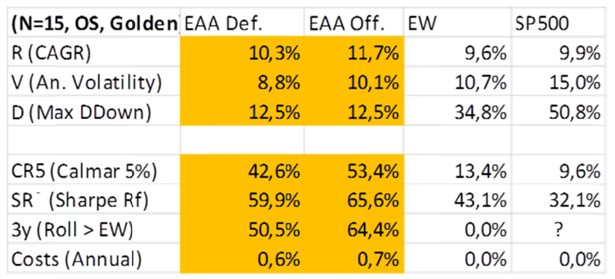
Why this table is shown as an image. It is not in the paper's text, only as an image, so the numbers for the 15-asset universe in the table above were copied from it.
What to notice. Both models have the same maximum drawdown, 12.5 %, against 34.8 % for equal weight and 50.8 % for the S&P 500. The share of three-year periods in which the defensive model beat equal weight is 50.5 %, that is, about half: on US sectors the defensive model's edge rests on drawdown, not on return.
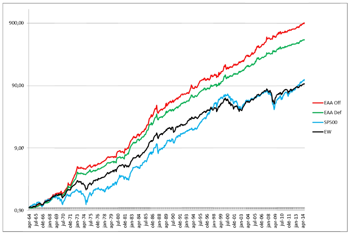
How to read it. The vertical axis is logarithmic: gridlines at 0.9, 9, 90 and 900, each ten times the previous one. On such an axis the same slope means the same percentage growth. The red line is the offensive model, green the defensive, light blue the S&P 500, black equal weight.
What to notice. Both EAA models are steadily above equal weight and the S&P 500 from the mid-1970s, and the gap widens over time. The dips on the light blue and black lines in 1974, 2002 and 2009 are barely visible for the EAA models; their most noticeable dip is around 1987.
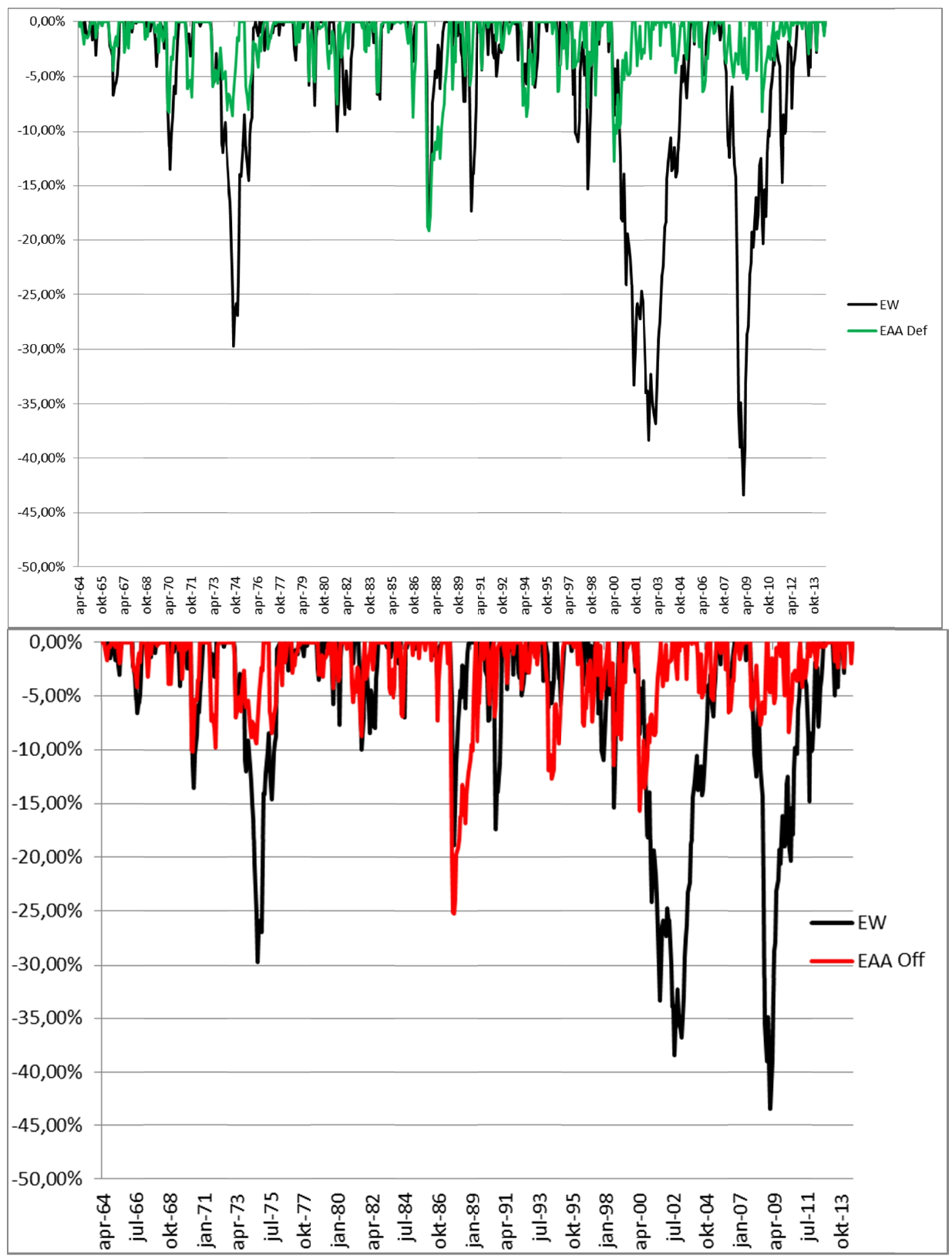
How to read it. Each line shows how far capital in a given month is below its previous high. Zero means a new peak. The deeper the dip, the larger the drawdown.
What to notice. Equal weight has three deep dips: about 30 % in 1974, about 38 % in 2002 and about 43 % in 2009. Both EAA models have small drawdowns in those periods. The models' deepest drawdown falls in October 1987: according to the paper's text, 19 % for the defensive and 25 % for the offensive. The next deepest is in May 2000, 13 % and 15 %. The rest, in the authors' words, are mostly no more than 10 %.
The practical takeaway. Absolute momentum protection on monthly data works in protracted bear markets and cannot react in time to a one-day crash. It was precisely a one-day crash that set the models' worst out-of-sample drawdown.
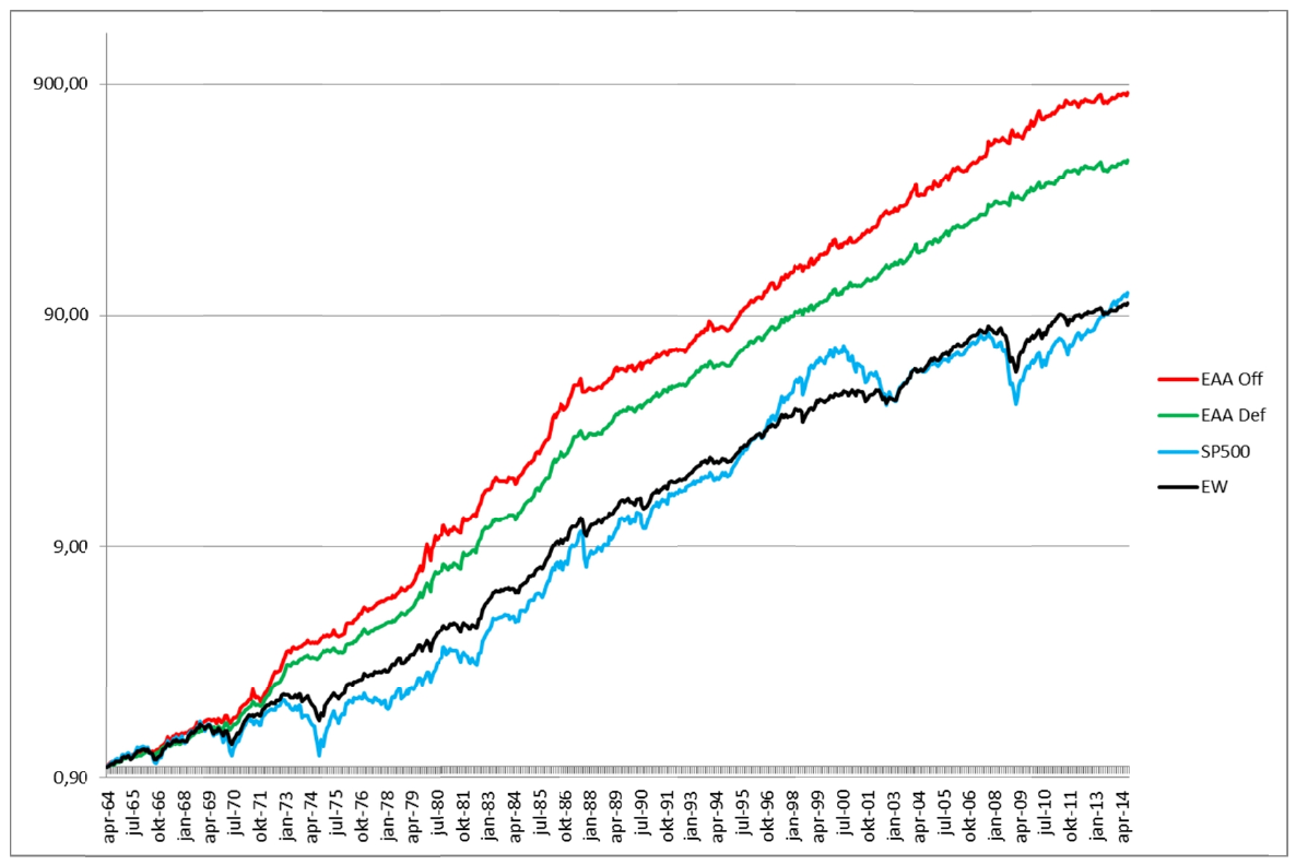
How to read it. The same logarithmic axis and the same colors as in the 7-asset figure.
What to notice. The EAA lines are smoother than on the small universe: the defensive model on this universe has an out-of-sample maximum drawdown of 8.6 % over 50 years, and, in the authors' words, all its drawdowns are below 10 %, including October 1987. All drawdowns of the offensive model are below 15 %. The authors call the result
"impressive in terms of its maximum drawdown (8,6% over 50 years OS)". Earlier, when discussing the Calmar metric (section 4.4 of the paper), they wrote that any multi-asset portfolio with a maximum drawdown of around 10 % over 100 years, like this defensive one on 38 indices, is"clearly exceptional".
The authors' conclusion from the out-of-sample test: on all three universes the golden models showed better absolute and risk-adjusted results than equal weight and the S&P 500. Hence their conclusion about the work of DeMiguel and co-authors, according to which the equal-weight portfolio compares favorably with optimized ones: "This conclusion is in contrast to the seminal article of DeMiguel (2007)". In their words, the advantage of optimization appears when the parameters are estimated tactically, over the last year.
Two more conclusions the authors draw in the conclusions section. The covariance matrix of size is replaced by two vectors of length : volatilities and correlations with the equal-weight index. And in the final models the main drivers turned out to be "return momentum and low beta (more precisely: low index correlation)".
10. What is shaky in the paper
The authors' own caveats
Drawdown as the optimization target. The first caveat on the authors' list: "Focusing on maximum drawdown effectively reduces sample size". Maximum drawdown is determined by a few large episodes, and fitting parameters to them, in the authors' words, "amplifies bias". Optimizing on Sharpe, they write, could be more informative and more familiar to the reader.
Timeliness of the old data. "Could the data have been compiled in a timely manner in the past?" During the training period and early in the test period, an index level may have become known with a delay of a week or a month, and this could have noticeably hurt the strategy. The authors suggest a test with a one-month delay but do not run it: "We leave this for subsequent research".
Friction in replicating the indices. There were no index-tracking funds at the start of the sample; had there been, "Frictions may have been very high", much higher than the assumed 0.1 % one-way, and the trading of such funds would itself have moved prices. The authors also write about the 0.1 % costs in the recipe: "This cost is realistic only for the most recent OS years". Footnote 6 contains a quick preliminary check: the offensive model on the 38-asset universe with costs up to 0.7 % one-way keeps its edge over equal weight on return, volatility and drawdown, and the authors conclude cautiously: "So there seems some room to allow for larger costs".
The recipe was fitted roughly. The recipe itself, in the authors' words, came from a “rough” optimization of on the training period with an eye to simplicity. Excess return in turned out to be only "marginally optimal".
The reason for dropping volatility is given as probable. The authors phrase the link to the collinearity of volatility and correlation with "probably"; the paper has no separate test of this explanation.
What is visible on reading but not discussed in the paper
These are our remarks, not caveats from the authors.
Out-of-sample by date, but not by the history of the idea. The authors write that with training only on 1914–1964 "there is no datasnooping involved". As far as the parameters' dates go, this is true. But the form of the model (a score from return, volatility and correlation, absolute momentum protection, monthly rebalancing) came from FAA and MAA, and those, as the paper itself says, were tested on daily data from recent decades, that is, inside the test period. The horizons of 1, 3, 6 and 12 months are justified by references to literature built on the same years. The test period is free of fitting numbers, but not of choosing the design.
How many variants there were in total is not stated. The number 49 refers only to the grid of the two exponents. Beyond them, the training period was also used to choose the return horizons, excess or nominal return, the rule for the number of assets, the safe asset, and the conclusions also mention a "cursory analysis to specify universe selection". The total number of combinations tried is not given, and the result cannot be corrected for the number of trials from the text.
The safe asset was chosen in one regime and worked in another. 10-year US Treasuries won on 1914–1964. In the test period, from the early 1980s to 2014, there was a long bond rally on falling rates, the very regime the authors were moving away from when they chose the training period. How much of the out-of-sample result comes from the protective share in bonds, the paper does not show separately.
The “38-asset” universe almost never had 38. On the training period it held 4 to 28 assets, all 38 are available only from 1994 to mid-2011, and by 2014 there are 13. The US sector universe consisted of 2 assets in 1914, 4 in 1921, and has all 15 only from 1927. The authors disclose this and call it a test on expanding and contracting universes, but the comparison with equal weight over such periods is a comparison on a very small universe.
Persistence of volatility was in effect not tested in this paper. Conclusion 3 speaks of "persistence of short-term volatilities V and index correlations C". Yet in all tests , and volatility does not enter the final models. The conclusion rests on the earlier FAA and MAA papers (the same sentence contains "as was demonstrated for FAA and MAA"), not on EAA results.
On the small universe the out-of-sample drawdown is noticeably deeper than in training. The golden defensive model on 7 assets: 11.7 % on the training period and 19.1 % on the test period; the offensive one 19.7 % and 25.3 %. On 38 assets it is the other way round: 10.9 % and 8.6 %, 21.9 % and 14.1 %. A single drawdown figure from a single history carries poorly into the future, and this agrees with the authors' own first caveat.
What each layer contributes is not tested. The model consists of three parts: selection by score, weights proportional to the score, and crash protection. The paper has no comparison of “EAA without protection” or “protection on top of equal weight”, although the authors themselves write that the selection rule and the protection can be applied to any scheme. How much of the gap with equal weight comes from the score formula and how much from the move into bonds cannot be seen from the paper.
11. What follows in practice
Protection by the share of falling assets is useful in its own right. It can be applied to any portfolio of several asset classes: count the share of assets with non-positive excess return over recent months and move the same share into the safe asset. According to the paper's figures, on monthly data it cut off the protracted bear markets of 1974, 2002 and 2009 and did not help in October 1987.
Correlation with the equal-weight index is cheaper than a covariance matrix. For assets you need numbers instead of , and each is computed from 12 monthly observations. The authors show that the factor approximates the maximum diversification portfolio. This is a convenient way to bring diversification into a rotation strategy without solving an optimization problem.
Take parameters from a plateau, not from a peak. On the 7-asset universe all 49 exponent combinations gave a drawdown of 10 to 22 % against 54.9 % for equal weight. This means that most of the result comes from the design and the protection, not from the exact values of the exponents. Before trusting a particular pair, it is worth looking at how the result changes across the whole grid.
Recheck costs and delay. The authors themselves consider 0.1 % one-way symbolic for most of the history, and they did not run the one-month delay test. With annual costs of 0.4–0.7 % already at 0.1 % per trade, the models' turnover is substantial; on real ETFs and funds this check has to be done with your own costs.
Set the drawdown benchmark by the worst out-of-sample episode. Even the defensive model on the small universe fell 19 % out-of-sample in 1987, whereas on the training period its worst drawdown was 11.7 %. Monthly rebalancing does not protect against a one-day crash.
A test on data after 2014. The paper ends in August 2014. The models are fully specified, and they can be run on the following years as a genuine out-of-sample test, without any fitting.
12. Testable ideas
| No. | Idea | Type | Where to compute |
|---|---|---|---|
| 1 | Run both golden EAA models unchanged on ETFs or indices after August 2014 and compare with the equal-weight portfolio of the same universe on R, D, CR5 and the share of three-year periods ahead | diagnostic | backtester |
| 2 | Execute rebalancing with a one-month delay, as the authors themselves suggest, and measure the loss of return and the increase in drawdown | acceptance metric | backtester |
| 3 | Run the model with costs of 0.1, 0.3 and 0.7 % one-way and find the threshold at which the edge over equal weight disappears | acceptance metric | backtester |
| 4 | Break the result down by layer: equal weight; equal weight plus protection by the share of falling assets; selection of the best without protection; full EAA | diagnostic | Python |
| 5 | Replace the safe asset, 10-year Treasuries, with bills and compute how much of the out-of-sample edge comes from the 1981–2014 bond market | audit | Python |
| 6 | Build a CR5 map over the whole 7 × 7 grid of and values on your own data and check whether the golden pairs sit on a plateau or on an isolated peak | audit | Python |
| 7 | Put volatility back into the score ( = 0.5 and 1) and compute the correlation between and across the assets of the universe to test the authors' collinearity explanation | diagnostic | Python |
| 8 | Choose the exponents by Sharpe instead of the Calmar ratio on the same training period and compare the chosen pairs and the out-of-sample result | audit | Python |