How to read this walk-through. The paper's method can be described without a single formula: split the history into chunks, divide the chunks in half many times, pick the best variant on one half and see where it landed on the other. That is the section “The method in one line”. Everything else explains what can be read from this and where the method misleads. Discrepancies with the text of the paper are in section 6.
The main thesis
When a researcher tries many variants of a strategy and picks the best one by backtest, the high Sharpe of the best variant says almost nothing: among thousands of variants on a finite history a lucky one will always turn up. The authors propose a question that can be answered with a number: with what probability does the variant that is best in-sample turn out worse than the median out-of-sample. That is PBO, the probability of backtest overfitting.
Estimating it does not require knowing how the strategy works. The matrix of returns of all variants in the search is enough. The CSCV procedure (combinatorially symmetric cross-validation) splits the history in half many times, in every possible way, and each time looks at where the winner lands. Unlike a single held-out chunk of data (hold-out), it uses the whole history and does not depend on which chunk happened to be held out.
In their example, a search over 8,800 rules of the form “which day of the month to enter and how long to hold” on a pure random walk gives a best variant with an annual Sharpe of 1.27, and PBO of 55 %. The same search on a series with a built-in seasonal effect gives PBO of 13 %.
1. How the problem is set up
A researcher has run variants of a strategy on one history of observations: different moving average lengths, thresholds, stops. Each variant has a return series. The researcher picks the best one by Sharpe. The question is not whether the best variant is profitable in-sample (it is, by construction), but whether the selection process keeps its advantage on new data.
The authors define overfitting not through a model but through ranks: a selection process is overfit if the variant that is best in-sample (IS) is expected to land out-of-sample (OOS) below the median of all variants. An important caveat from the authors themselves: this is about overfitting of the selection process, not about the calibration of a single model. That is why the definition does not require knowing what is inside the strategy.
The authors list five reasons why an ordinary held-out chunk of data does not work. The short one: if the researcher tried more than one variant, overfitting is always present, and a hold-out does not account for the number of attempts. The others: the researcher has seen public data anyway; on short series the held-out chunk is small; holding out the end of the series loses the most recent data; different held-out chunks lead to different conclusions.
2. The method in one line
Split the history into equal chunks, go through every way of choosing half of the chunks for training, find the best variant on each and look at its rank on the remaining half. PBO equals the share of splits where that rank is below the median.
Step by step, as in algorithm 2.3 of the paper:
- Build a matrix of size : each column holds the returns of one variant, and the rows are synchronous.
- Cut the rows into an even number of chunks of equal length.
- Go through all combinations of the chunks taken at a time. Each combination is a training half ; the remaining chunks are the testing half .
- On the training half, compute the Sharpe of every variant and find the best one, .
- On the testing half, compute the Sharpe of all variants and determine the relative rank of : , a number between 0 and 1.
- Convert the rank to a logit: .
- PBO is the share of combinations where , that is, where the rank is no higher than the middle.
What this is. The number of ways to choose half of the chunks. The check is repeated this many times.
What each symbol means. (ess): the number of chunks. (factorial): the product of all numbers from 1 up to the given one.
A worked example on the paper's numbers. With (chunks A, B, C, D) there are six combinations: AB against CD, AC against BD and so on; this is figure 1 of the paper. With there are 12,870, and with already 2,704,156.
Why this matters. Each half serves exactly once as training and once as testing, and both halves have the same length. So the comparison is fair: the in-sample and the out-of-sample Sharpe are estimated on the same amount of data.
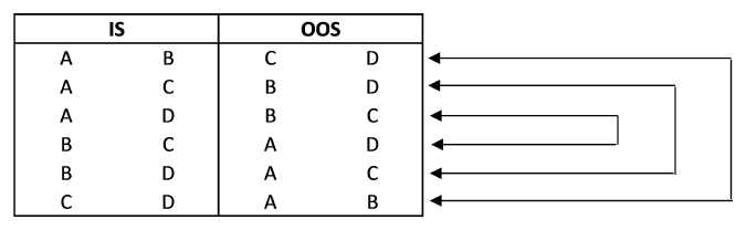
How to read it. Each row is one combination: on the left, the two chunks on which the best variant is chosen (IS); on the right, the two on which it is tested (OOS). The arrows show that each combination also appears in the reverse role.
What this is. A logit: it maps the rank from the interval between 0 and 1 onto the whole number line. Zero means the median, plus means above the median, minus below it.
Step by step, our example. Out of 880 variants, the winner of the training half took 700th place from the bottom on the testing half. Then , : good. Had it taken 300th place, , : this case counts toward PBO.
Why this matters. The distribution of logits across all combinations shows the whole picture: where the center is, how wide the spread is, whether the left tail is long.
The authors recommend : with four years of daily data the chunks come out as quarters, and 12,870 combinations are enough to estimate the share with a precision of about 0.01. The number of variants should be well above ten, otherwise the ranks take too few values.
3. What else the same procedure gives
Besides PBO, the same combinations yield three more things.
Degradation. Pairs of “the winner's in-sample Sharpe, the same winner's out-of-sample Sharpe” across all combinations. Regressing the second on the first usually gives a negative slope: the higher the in-sample Sharpe, the lower the out-of-sample one. The authors explain this by the overfit model being tuned to the noise of the past and therefore less prepared for the future.
Probability of loss. The share of combinations where the winner has a negative out-of-sample Sharpe. The authors stress that it can be high even when PBO is low; in that case the strategy is bad for reasons unrelated to overfitting.
Stochastic dominance. A comparison of the distribution of out-of-sample Sharpe among the winners with its distribution among all variants. If the winners do not dominate, the selection procedure is no better than picking a variant at random.
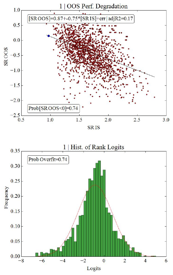
How to read it. At the top, each point is one combination: horizontally, the winner's in-sample Sharpe; vertically, its out-of-sample Sharpe. At the bottom, a histogram of logits. Labels inside the figure:
Prob[SR OOS<0]=0.74andProb Overfit=0.74.What to notice. All in-sample Sharpes are between 1 and 3, while out of sample the cloud slopes downward at −0.75. The logits are shifted to the left of zero.
The practical takeaway. An in-sample Sharpe of 2–3 under such a selection process promises nothing: out of sample, three quarters of the winners lose money.
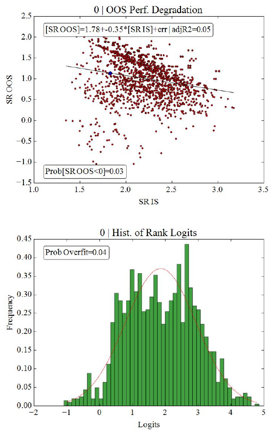
How to read it. The same two panels for a “real investment strategy” that the authors do not describe. Labels:
Prob[SR OOS<0]=0.03,Prob Overfit=0.04.What to notice. The cloud is above zero, the slope is −0.35, the logits are almost entirely on the right. There is a negative slope here too: degradation is inherent in any selection; the question is how strong it is.
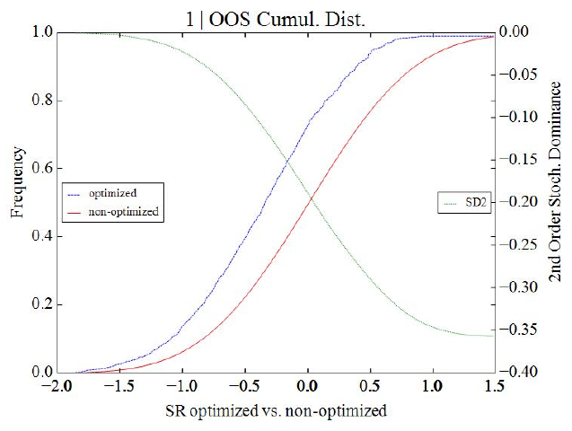
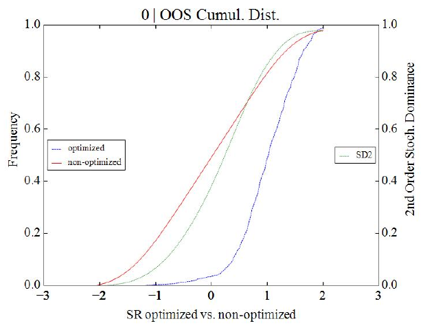
How to read figures 4 and 5. Two distribution functions of out-of-sample Sharpe: for the winners (optimized) and for all variants (non-optimized), plus a second-order dominance curve. In figure 4 the winners' curve lies to the left, meaning that selection does harm. In figure 5 it lies to the right: selection really does find something better.
4. A practical example
A seasonal rule: which business day of the month to enter on (1–22), how many days to hold (1–20), a stop measured in volatilities (in the paper, an interval from 0 to 10), long or short. In total, according to the authors, 8,800 variants. A series of 1,000 daily prices, about four years.
On a pure random walk the best variant (enter on day 11, hold 4 days, stop −1, long) gives an annual Sharpe of 1.27 and a PSR statistic of 2.83, that is, less than a 1 % chance that the true Sharpe is below zero. Judging by this backtest alone, the strategy looks significant. CSCV gives the following: in 53 % of combinations the winner loses money out of sample, PBO is 55 %, there is no dominance. The method correctly diagnoses overfitting, since a random walk has no seasonality.
With a built-in effect (the first five days of every month shifted by a quarter of a standard deviation) the best variant (enter on day 1, hold 4 days, stop −10, long) gives a Sharpe of 1.54, almost the same. But out of sample only 13 % of the winners lose money, PBO is 13 %, and there is dominance.
The authors' moral: the high in-sample Sharpe is the same in both cases; only PBO tells them apart.
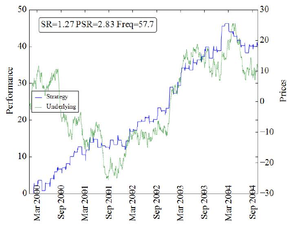
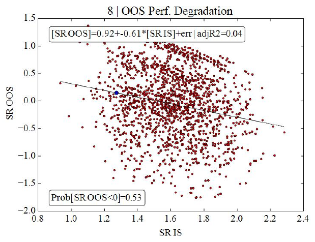
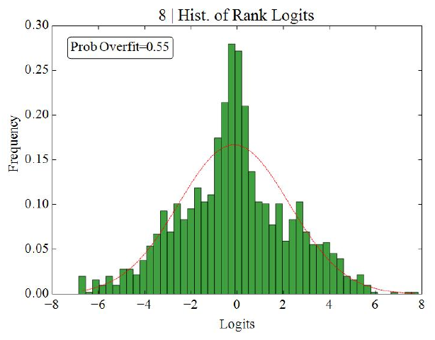
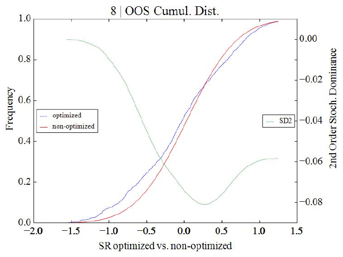
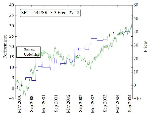
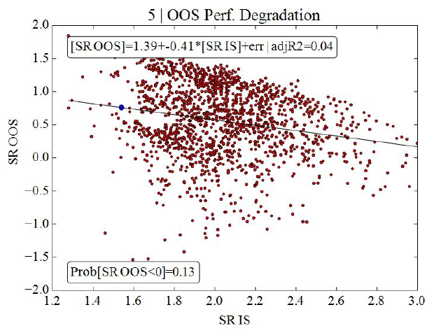
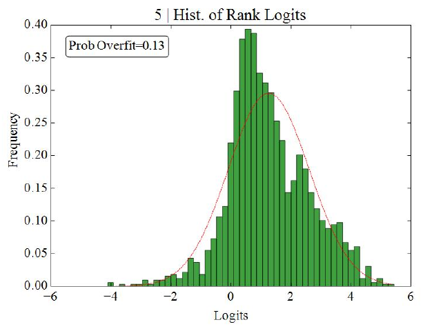
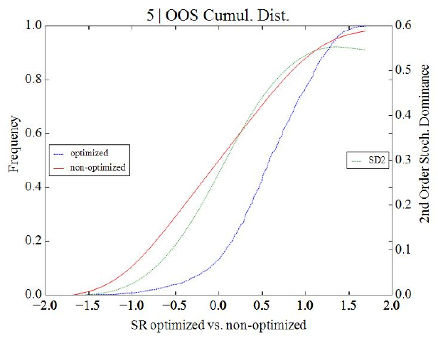
How to read figures 6–13. Figures 6 and 10: the blue step line is the cumulative result of the best variant, the green line is the price of the series. Both look like a good strategy. Figures 7 and 11: the cloud of Sharpe pairs; in the first case the center of the cloud is near zero, in the second near one. Figures 8 and 12: the logits; in the first case the center is at zero, in the second it is shifted to the right. Figures 9 and 13: in the second case the winners' curve lies to the right.
The practical takeaway. Overfitting cannot be seen on the equity curve of the best variant. It shows only in a comparison with the other variants on the other half of the data.
Our check on our own series
We wrote CSCV following algorithm 2.3 and repeated the experiment on ten random series of the same construction: 1,000 days, an “entry day × holding period × side” grid without a stop, 880 variants, .
| Series | PBO across ten series | Mean | Paper, one series |
|---|---|---|---|
| Random walk | 0.39 … 0.69 | 0.60 | 0.55 |
| First 5 days shifted by +0.25σ | 0.01 … 0.36 | 0.19 | 0.13 |
The paper's qualitative conclusion reproduces: with an effect, PBO is noticeably lower. But something the paper does not discuss is also visible: PBO from a single series varies a lot from one series to the next (section 6).
5. Limitations the authors name themselves
Section 5 of the paper is honest and useful, and it is worth retelling closely.
Design. Splitting strictly in half and into equal chunks does not suit every strategy; with strong autocorrelation of results and a large , the chunks break the structure. All combinations carry equal weight; if something is known about the distribution of results, special schemes may be more accurate.
Application. All trials must be disclosed: "Hiding trials will lead to an underestimation of the overfit". Nor may deliberately failing variants be added to make the winner look better. For a directed search (an optimizer that decides by itself where to go next), the matrix receives the final solution of each search, not the intermediate steps.
The procedure "does nothing to evaluate the correctness of a backtest": it does not catch wrong costs or look-ahead.
It does not see a structural break outside the available history.
A high PBO does not mean there are no good strategies: if all variants are equally good, the winner is random, and PBO is high among strategies that are all "skillful".
And the main warning: PBO must not be used as an optimization objective; that "would constitute a gross misuse of our method". Any device against overfitting that becomes a selection criterion starts overfitting itself.
6. What is shaky in the paper
What turned up in the cross-check
1. The number of combinations at . The text has "if S = 16, we will form 12, 780 combinations". By formula (2.3) of the paper, . The other combination counts in the paper are correct (924 at , 2,704,156 at ). A typo that does not affect the precision estimate: and , both below the stated 0.0045.
2. The PBO of the real strategy is understated a hundredfold in one of two places. In section 3.2 it is first "was only 4%", and a paragraph later "with a PBO of 0.04%". Figure 3 itself shows Prob Overfit=0.04, that is, a share of 0.04, or 4 %. The first is correct.
3. The share of negative Sharpes in the example of figure 2. The text has "about 78% of the SR OOS are negative". The label on the figure is Prob[SR OOS<0]=0.74. The rendering was checked at 300 dpi.
4. In the conclusions the definition of PBO is switched from the median to the mean. Definition 2.2 and the whole text speak of a rank below the median. Section 7 has: "the probability that an optimal strategy IS underperforms the mean OOS". For a distribution of Sharpes with tails, the median and the mean differ, and these are two different criteria.
5. The logit of a uniform rank is not standard normal. Section 4: "the distribution of the logits will approximate the standard Normal". The logit of a uniformly distributed variable follows the standard logistic distribution; its standard deviation is , not 1. Our calculation on a million uniform numbers: 1.813. The shape resembles the normal one, but the scale is almost twice as wide. This matters if anyone wants to compute the “significance” of the mean logit on a normal scale.
6. Step c) of the algorithm mixes up the samples. "the nth column of J (the testing set)": in step a) is defined as the training half, and the testing half is from step b). The context makes it clear that the training half is meant; when the algorithm is rewritten as code, this line is misleading.
A minor point. The grid of the example does not add up: "the interval [0, . . . , 10] for Stop loss" gives 11 values, and then , not "8,800 elements"; 8,800 comes out with ten stop values (the winners have stops of −1 and −10). It does not affect the conclusions.
What a check shows but the paper does not discuss
The precision of PBO is overstated. The authors estimate the error of the share as if the trials were independent: with 12,870 combinations the standard deviation is below 0.0045, and "less than a 0.01 estimation error at 95% confidence level". But the combinations overlap, each shares chunks with thousands of others, and they are not independent. Most importantly, this precision describes the spread across the combinations of one history, not how much PBO depends on the history itself. On our ten random walks, PBO for one and the same process ranges from 0.39 to 0.69, and with an effect from 0.01 to 0.36. A single PBO figure from a single history is uncertain by tens of percentage points. Our calculation.
In a grid with mirrored variants, PBO coincides with the probability of loss. If for every rule the search contains both a long and a short (the authors have a Side parameter), the median out-of-sample Sharpe is near zero, and “below the median” is almost the same as “losing money”. That is why the authors' pairs of numbers are so close: 55 % and 53 %, 13 % and 13 %. On our grid they matched to the hundredth: 0.60 and 0.60, 0.19 and 0.19. In this case the two metrics carry no independent information. Our conclusion.
The 0.05 threshold is stricter than it looks. The authors allow one to "reject models for which PBO is estimated to be greater than 0.05". Given the spread of PBO across histories shown above, a 0.05 threshold on one history is almost unreachable for a strategy with a weak real effect: for our series with real seasonality, PBO came out below 0.05 in one case out of ten.
The “real strategy” is not described. Figures 3 and 5 are given without a description of the strategy, the data or the number of variants. They cannot be checked.
7. What follows in practice
Store every variant in the search, not just the best one. PBO can only be computed from the full return matrix. An optimizer that keeps a single winner makes the method impossible to apply after the fact. In practice this means saving the daily results of every grid configuration, not just the final result of the best one.
Read a PBO figure from one history as a rough estimate. The spread between histories is comparable to the value itself. It is more reliable to compute PBO on several instruments or periods and look at the spread.
Report the negative slope of “out-of-sample Sharpe against in-sample Sharpe” next to the best result. It is the most visual part of the method and the cheapest: the same search, one regression.
Do not choose a strategy by PBO. This is a direct warning from the authors. PBO assesses the selection process, not the strategy.
For prop problems. Choosing size and settings to fit evaluation rules is also a search over configurations (Hall, 2026, has 324 configurations in the adversarial test). If the best configuration is shown without where it lands on the other half of the history, the backtest pass rate means nothing.
8. Testable ideas
| No. | Idea | Type | Where to compute |
|---|---|---|---|
| 1 | Save the daily returns of all configurations of every search and compute PBO via CSCV with before choosing a finalist | acceptance metric | backtester |
| 2 | Keep a log of all trials for each strategy, including abandoned ideas: PBO from an incomplete set is understated, and the paper says so directly | audit | any |
| 3 | Compute PBO on several instruments or non-overlapping periods and report the spread; on a single history the value moves by tens of pp | acceptance metric | Python |
| 4 | Report the regression of “out-of-sample Sharpe on in-sample Sharpe” over the CSCV combinations next to the best result; the negative slope and the share of negative OOS | acceptance metric | Python |
| 5 | Check stochastic dominance of the winners over all variants: if there is no dominance, the selection procedure is no better than a random choice | audit | Python |
| 6 | In grids with mirrored (long/short) variants, do not count PBO and the probability of loss as two independent pieces of evidence: they coincide by construction | audit | any |
| 7 | For an optimizer with a directed search, put into the matrix only the final solutions of each run, not the intermediate steps | audit | Python |
| 8 | Compute the mean and spread of logits on the logistic scale (), not the normal one | audit | Python |