How to read this walk-through. The paper is short (14 pages) and careful. The core is in three tables: what each rule costs (section 3), the probability of reaching funding over a “skill × size” grid (section 4) and the fair fee (section 5). We reproduced the model independently; the result is in section 6.
Main thesis
A prop-firm challenge is a contingent claim with a posted price and hidden probabilities. The author values it the way an actuary would: the trader's equity is Brownian motion with drift, the target is an upper barrier, the overall limit a lower one, the daily limit a constraint on a single time step, the time limit is the maturity, and the funded account a stream of contingent payouts.
Three conclusions. Rules that look symmetric (+10 % target, −10 % limit) are not symmetric: the 30-day time limit and the daily limit turn a fair 50 % coin into 29.8 %, and almost all of that is the time limit's doing. The contract's value is concentrated on a narrow ridge of position size around 2 % daily volatility, and marketing is silent about it. With the given illustrative population the average value of a $500 challenge is $221, the firm's margin 56 %, and 7.5 % of buyers reach funding.
Hence the regulatory proposal: require firms to publish a cohort funnel, the ratio of payouts to revenue and the median payout.
1. How the contract works
| Parameter | Value |
|---|---|
| Account size | $100,000 |
| Price | $500, refunded with the first payout |
| Step 1 target | +10 % |
| Step 2 target | +5 % |
| Daily limit | 5 % of the initial balance |
| Overall limit | 10 % of the initial balance |
| Step 1 time limit | 30 trading days (variant: no time limit) |
| Step 2 time limit | 60 trading days (variant: no time limit) |
| Trader's share | 80 % |
| Payouts | every 20 trading days, balance reset |
| Funded-account horizon | 250 trading days |
| Monitoring | at daily closes |
Table 1 of the paper. This is a stylized “classic two-step” contract; no firm is reproduced exactly. The limits are static, measured from the initial balance, not trailing.
Skill is set by an annual Sharpe after costs, size by the daily volatility :
What this is. Each day equity changes by a random amount with mean and spread , as a fraction of the initial balance. Skill and size are kept apart: is the quality of the signal, how aggressively it is expressed.
Example, our calculation. A Sharpe of 1 at 2 % daily volatility: , about 0.13 % a day, or $126 on a $100,000 account.
Costs enter as a fraction of daily volatility: the annual Sharpe falls by . At the base that is 1.59, meaning a trader with a gross Sharpe of 1.59 has zero after costs.
2. The method in one line
Without the daily limit and the time limit, the probability of reaching before is known exactly:
What this is. The gambler's ruin formula for Brownian motion with drift: the chance of reaching the target before the limit.
What each symbol means. : the target as a fraction of the balance (0.10). : the limit as a fraction (0.10). (theta): the ratio of drift to variance, doubled. : the base of the natural logarithm.
Step by step on the paper's numbers. Sharpe 2, volatility 2 %: , , . Then . The paper has 0.779. At the formula turns into .
Why this matters. It is a ceiling: everything the rules add only lowers it. The same formula appears in Villahermosa (2026) and Hall (2026).
The rest is computed by Monte Carlo: 200,000 paths per cell, a grid of 12 Sharpe values from −5 to +4 and five volatilities from 0.5 % to 5 %.
The fair fee with the fee refund:
What each symbol means. : the probability of reaching funding. : the expected sum of payouts once funded. : the probability of at least one payout once funded; the fee is refunded with exactly that payout.
What this is. The fee at which the buyer's expectation is zero. The fee refund makes the fee partly self-canceling: part of any markup on the fee comes back to whoever reaches the first payout.
A worked example on the paper's numbers. Zero edge, 2 % a day: the funding probability is 0.184, expected payouts once funded about $7,300, a first payout in 56 % of cases. ; the paper has $1,502 (the payouts are given rounded).
3. What each rule costs
| Rule set | Sharpe 0 | Sharpe +2 |
|---|---|---|
| Barriers only (formula) | 0.500 | 0.779 |
| + daily limit | 0.453 | 0.744 |
| + 30-day time limit | 0.310 | 0.550 |
| + both (base contract) | 0.298 | 0.532 |
Table 2 of the paper, step 1, volatility 2 %. The daily limit takes 4.7 pp from a trader with no edge, the time limit 19.0 pp. The “+10 / −10” symmetry promises a coin flip, and with the rules it comes out at 30 %. Removing the time limit brings it back to 45.3 %.
4. Size matters as much as skill
| Sharpe | 0.5 % | 1 % | 2 % | 3 % | 5 % |
|---|---|---|---|---|---|
| −3.0 | <0.001 | 0.001 | 0.022 | 0.046 | 0.070 |
| −1.0 | <0.001 | 0.008 | 0.100 | 0.128 | 0.130 |
| 0.0 | <0.001 | 0.026 | 0.184 | 0.195 | 0.172 |
| +1.0 | <0.001 | 0.066 | 0.298 | 0.278 | 0.220 |
| +2.0 | 0.001 | 0.135 | 0.434 | 0.375 | 0.275 |
| +3.0 | 0.004 | 0.241 | 0.576 | 0.471 | 0.334 |
Part of table 3 of the paper: the probability of passing both steps. A trader with a Sharpe of +1 at 0.5 % volatility almost never reaches funding, because 30 days are not enough to get there. A trader with a Sharpe of −1 at 2 % gets there in 10 % of cases. The author: "The contract cannot distinguish a modestly skilled cautious trader from an unskilled aggressive one".
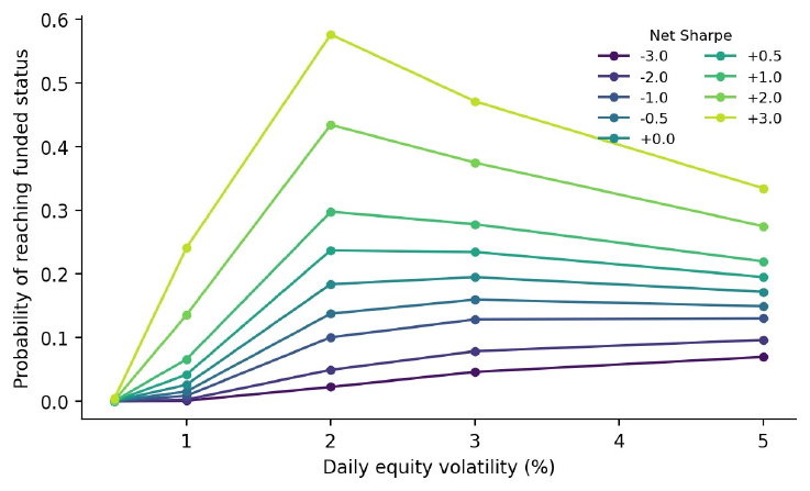
How to read it. Horizontally, daily volatility in percent; vertically, the probability of passing both steps. Each line is one Sharpe after costs, from −3 (dark) to +3 (light).
What to notice. All lines with a non-negative Sharpe peak around 2 %, the negative ones around 3–5 %. On the left all lines are pinned to zero.
The practical takeaway. Too cautious a size kills the chance faster than a lack of skill: the trader does not get there before the time limit runs out.
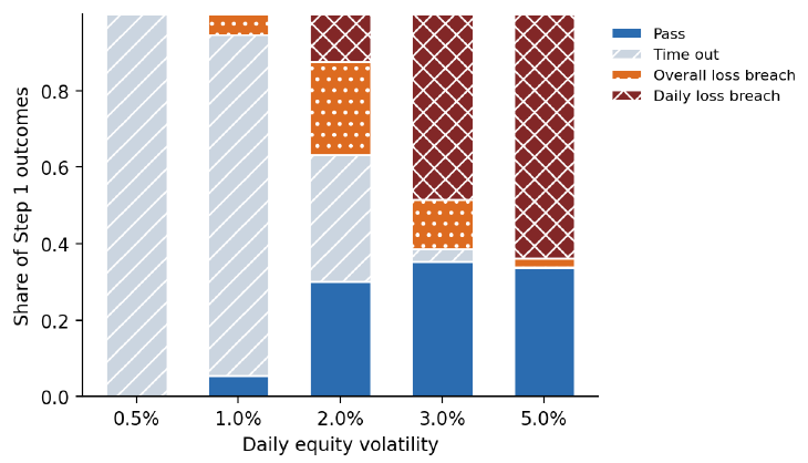
How to read it. One bar per volatility, with the shares of step 1 outcomes: pass, time limit expired, overall limit, daily limit.
What to notice. At 0.5 % and 1 % almost everything is the time limit expiring. At 3 % and 5 % almost everything is a breach of the daily limit. The pass share peaks in the middle.
The practical takeaway. The ridge is formed by two different ways of losing. The time limit punishes small size, the limits punish large size.
5. The fair fee and the ridge
| Sharpe | 0.5 % | 1 % | 2 % | 3 % | 5 % |
|---|---|---|---|---|---|
| −1.0 | 0 | 27 | 404 | 280 | 58 |
| −0.5 | 0 | 72 | 783 | 457 | 85 |
| 0.0 | 0 | 183 | 1,502 | 728 | 127 |
| +0.5 | 1 | 432 | 2,790 | 1,143 | 184 |
| +1.0 | 2 | 979 | 5,058 | 1,730 | 263 |
Part of table 4 of the paper, in dollars. At a price of $500 and 2 % volatility a Sharpe of −0.87 already breaks even: "the contract forgives skill deficits of nearly one Sharpe unit". At 1 % it takes +0.56, at 5 % +1.94, and at 0.5 % no Sharpe on the grid is enough. Our recount by interpolation over table 4: −0.87 and +0.56 match exactly; for 5 % linear interpolation gives +1.87, and the exact root on a convex curve lies further right, so +1.94 is plausible.
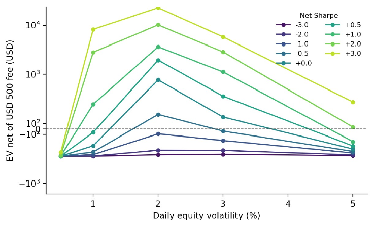
How to read it. Horizontally, daily volatility; vertically, the buyer's expectation net of $500. The scale is symmetric-logarithmic: linear from −1,000 to +1,000, logarithmic beyond. The dashed line is zero.
What to notice. All lines peak around 2 %. The Sharpe −0.5 line is above zero only there; the Sharpe 0 and +0.5 lines are above zero at 2–3 %, the +1 line already from 1 %. At 0.5 % all lines are below zero.
The practical takeaway. The firm's margin, in the author's words, comes not so much from buyers with no skill as from costs and from buyers who do not trade on the ridge.
6. The population and sensitivity
The illustrative population: gross Sharpe standard normal, minus 1.59 for costs; sizes on the volatility grid with weights of 5/20/30/25/20 %.
| Quantity | Value |
|---|---|
| Average value, with refund | $221 |
| Same, without refund | $203 |
| No time limit (without refund) | $369 |
| No costs | $1,098 |
| Firm's margin | $279 (56 %) |
| Share reaching funding, classic / no time limit | 7.5 % / 10.5 % |
Table 5 of the paper. The author stresses this: "These are model outputs under stated assumptions, not estimates from challenge-account data". Table 6 varies costs and the size distribution: from $60 to $557.
Our check: the model is reproduced
We wrote the model from sections 4–5 of the paper without the author's code. The result:
| What | Paper | Ours |
|---|---|---|
| Table 2, Sharpe 0: daily limit / time limit / both | 0.453 / 0.310 / 0.298 | 0.456 / 0.308 / 0.299 |
| Table 2, Sharpe 2 | 0.744 / 0.550 / 0.532 | 0.743 / 0.549 / 0.534 |
| Table 3, Sharpe 0, volatility 1 / 2 / 3 / 5 % | 0.026 / 0.184 / 0.195 / 0.172 | 0.025 / 0.181 / 0.196 / 0.173 |
| Table 4, Sharpe +1 | 979 / 5,058 / 1,730 / 263 | 976 / 5,076 / 1,733 / 269 |
| (first payout | funded), Sharpe 0, 2 % | 0.56 | 0.56 |
| Share reaching funding in the population | 7.5 % | 7.52 % |
| Average value without refund | $203 | $203 |
| Fee-refund contribution | $18 | $9 |
Everything except the refund contribution matches within Monte Carlo error. Our refund contribution is half as large. The reason shows up cell by cell: at 5 % volatility (a weight of 20 % in the population) funded accounts almost always die before the first payout, and our average probability of a first payout across all funded accounts is 0.24, while $18 needs about 0.48. We checked an alternative reading (“the refund is paid if the account survived to the first payout date, even without profit”): $12, also not $18. Without the author's code the cause cannot be established. It barely affects the conclusion: an average value of $212 instead of $221, a margin of 58 % instead of 56 %.
7. The regulatory proposal
The author proposes not to ban the product but to require disclosure for each product and rule version, quarterly: a cohort funnel (challenges bought → step 1 → step 2 → first payout → repeat payout) with challenges bought in the denominator and resets counted as new purchases; the ratio of payouts to fee revenue, with refunds treated explicitly; the median payout among those who received one. Plus a warning that the chance of passing depends strongly on position size, modeled on the leverage warnings for CFDs. The templates: the disclosure of the share of losing accounts for CFDs in the EU (ESMA 2018) and the return-to-player figure for slot machines in the UK.
Separately, the paper examines the regulatory position of the Czech National Bank (2023): a simulation without execution is usually not an investment service, but a reward that depends on demo results may require assessment under derivatives law. That is exactly the contract the paper values.
8. What is shaky in the paper
What the author admits
Six limitations are listed directly. Returns are normal and independent; with a Student distribution (4 degrees of freedom) the pass rate at 2 % falls from 0.298 to 0.273. Monitoring is at daily closes, while many firms monitor intraday, so all values are an upper bound. The trader is mechanical, with constant size. Consistency rules, payout caps and payout denials are not modeled, and this again shifts the estimates upward. The 250-day horizon cuts about 8 % of the value at a Sharpe of 2. The population is set by assumptions.
What our check turned up
1. “Eight of nine” is in fact seven of nine. In section 6.4: "The posted fee exceeds the model-implied average value in eight of nine scenarios". In table 6 at two values are above $500: 557 and 517. The price exceeds the value in seven scenarios out of nine. The author's very next sentence ("only when trading costs are at the low end (k = 0.05) does average value approach or exceed USD 500") agrees with the table, so the error is in the count, not in the conclusion.
Not reproduced. The $18 fee-refund contribution (section 6 above). This is not a proven error: without the author's code we cannot rule out an implementation detail that is not in the text.
Minor points. Section 8 refers to "Tables III and IV", although the tables are numbered with Arabic numerals (3 and 4). In the abstract, “0.30” refers only to step 1; the probability of passing both steps at the same point is 0.184, and the abstract does not make that visible.
What a check shows but the paper does not discuss
There is no payout cap, and the sign depends on it. The author models 80 % of all profit every 20 days with no cap. In Hall (2026) the cap is $1,000 per cycle, and the expectation is negative for any realistic trader; here, on the ridge, the expectation is not below zero from a Sharpe of −0.87 upward. The author notes that caps are not modeled and that this shifts the estimates upward, but does not show by how much. Per Hall, doubling the cap from $1,000 to $2,000 changes the hedged pair's expectation from +$9 to +$215: this is the main parameter, not a correction.
The population determines the result. $221, 56 % and 7.5 % rest on two assumptions with no data behind them: the skill distribution and the size distribution. Table 6 shows a spread from $60 to $557. The author says so, but the abstract gives exactly the point figures.
9. What follows in practice
Before buying a challenge, compute your own “probability × size” surface. With static limits and a time limit the ridge always exists: too small a size does not get there in time, too large a size knocks out the daily limit. For the classic 10/10/5 over 30 days it is about 2 % a day, that is, $2,000 on a $100,000 account.
The time limit costs more than the daily limit. 19 pp against 4.7. In the model the version without a time limit is worth $369 to the population against $203 for the classic (both without refund), so a price markup of up to $166 pays for itself on average (our calculation from table 5). The author shows that removing the time limit closes 56 % of the gap between value and price.
Costs as a fraction of daily volatility. If costs eat 10 % of the daily swing, that is minus 1.59 of annual Sharpe. For frequent trading on CFDs this is a real magnitude, and it is worth measuring on your own strategy before buying.
10. Testable ideas
| No. | Idea | Type | Where to compute |
|---|---|---|---|
| 1 | Build a “funding probability × daily volatility × Sharpe” surface for a specific firm's rules and choose a size on the ridge before buying | diagnostic | Python |
| 2 | Break down the loss of pass probability by rule (time limit, daily limit, overall limit), adding them one at a time, as in table 2 of the paper | diagnostic | Python |
| 3 | Compute the fair fee with the fee refund and compare it with the price, not with zero | acceptance metric | Python |
| 4 | Measure the strategy's costs as a fraction of daily volatility and convert them into a Sharpe correction | diagnostic | Python |
| 5 | Check the size ridge with intraday limit monitoring and with heavy tails; in the author's run at t(4) the pass rate falls from 0.298 to 0.273 | audit | Python |
| 6 | Add a payout cap and consistency to the model and show how much the sign of the expectation changes; the paper leaves them out | design change | Python |