How to read this walk-through. The paper answers two questions: which of the index and two ETFs on it leads, and by how many milliseconds, and how this lead changes on days when new information arrives. The lead-lag measurement method, which is useful for any pair of instruments with non-synchronous trades, is taken apart in sections 2 and 3 with formulas and numbers. The results are in sections 5 and 6. If you need only the practical conclusion, read sections 7, 8 and 9: the trading test in the paper is a single sentence, and you should know this before citing it.
1. How the problem is set up
Lead-lag is the situation when one instrument repeats the moves of another with a delay. If the market were efficient and frictionless, related instruments, for example an index and a fund tracking that index, would have returns coinciding in time. In practice lead-lag is found all the time, especially between a future and an index. The paper's literature review gives benchmarks from older studies: the future leads the index by up to 45 minutes, the index leads the future by no more than 15 minutes; at the same time Brooks and coauthors (2001) found that accurate forecasts based on lead-lag do not beat a benchmark after costs.
The authors take three instruments on one and the same index: the S&P 500 itself and the two most liquid ETFs on it, SPY (State Street) and IVV (BlackRock). All three trade electronically and all are spot, so the explanations through different trading costs and different trading mechanisms (electronic or floor), which the literature used to explain the lead of the future, do not apply here, in the authors' view. What remains is the speed with which the instruments reflect new information.
The measurement has to be done on ticks, not on bars. The authors refer to Huth and Abergel (2014): electronic trading has shortened the lag so much that data on a regular grid no longer catch it. But on ticks another problem arises: trades in the two instruments happen at different moments, and they cannot be aligned to a grid without distortion.
What the Epps effect is. The observation by Epps (1979): the more frequently prices are sampled, the lower the correlation between instruments, even between nearly identical ones. An index and a fund on it correlate at 99.9 % on daily data, and at about 20 % on ticks. The causes are the non-synchronicity of trades and the fact that on a very short scale common information has not yet reached both prices.
2. The method in one line
Compute the correlation of two tick series without aligning them to a grid (multiply returns only on overlapping intervals between trades), then shift one series in time in steps of 10 ms and look for the shift at which the correlation is highest. The position of the peak is the lead-lag time, the height of the peak is the lead-lag correlation, and the asymmetry of the whole curve is the lead-lag ratio.
The methodology is taken from Alsayed and McGroarty (2014): the correlation of Hayashi and Yoshida (2005), its extension to shifts by Hoffmann, Rosenbaum and Yoshida (2013), and the lead-lag ratio of Huth and Abergel (2014). The paper's contribution is not in the method but in computing these three quantities for each day and explaining them by daily volume.
3. How lead-lag is computed
3.1 Correlation without alignment
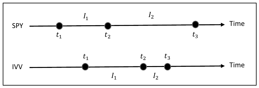
How to read it. Two time axes. The points are the moments of trades, is the arrival time of an observation, is the interval between two adjacent trades of one instrument.
What to notice. SPY and IVV trade at different moments, and the intervals have different lengths. Taking “the return over the same second” for both is impossible: within a second one may have many trades and the other none.
What this is. The Hayashi and Yoshida covariance: formula (1) of the paper.
What each symbol means. (“R SPY on the i-th interval”): the return of SPY between two of its adjacent trades. : the same for IVV on its interval. : an indicator, equal to 1 if the intervals overlap in time even slightly, and 0 if not. (“intersection”), (“empty set”): the notation reads “the intervals have a common part”.
Step by step. Go through all pairs “SPY interval, IVV interval”. If they overlap, multiply the returns and add to the sum. If not, skip. No filled-in points.
An example from figure 2. The authors list the overlapping pairs: (, ), (, ) and (, ). The first SPY interval is short and touches only the first IVV interval; the second is long and touches both.
What this is. Formulas (2)–(4) of the paper: the “standard deviation” of each series as the square root of the sum of squares of its own returns, and the correlation as the covariance divided by their product. Each series is computed over its own intervals, without synchronization.
A worked example (our example). SPY returns on two intervals are +0.02 % and −0.01 %, IVV +0.03 % and −0.02 %, the overlaps as in figure 2. Covariance . Deviations and . Correlation .
Why this matters. This is the standard way to compute the correlation of a pair with non-synchronous trades. Interpolation and alignment to a grid, according to the authors, introduce biases that this method avoids.
3.2 The shift and the correlation curve
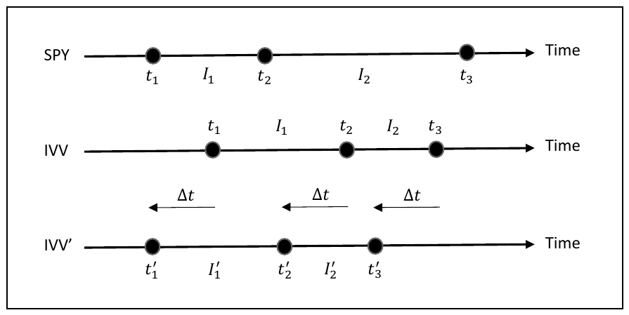
How to read it. IVV' is a copy of the IVV series in which every observation is shifted back in time by the same amount . Then the correlation is recomputed between SPY and IVV'.
What to notice. If IVV repeats SPY with a delay, shifting IVV back aligns the reaction with its cause, and the correlation rises. The shift at which it is highest is the lag.
What this is. Formula (5) of the paper: the same Hayashi–Yoshida correlation, but with the shifted series. The prime means “after the shift”; checks the overlap of SPY intervals with the already shifted IVV intervals.
How the curve is built. is recomputed for from −100 to +100 ms in steps of 10 ms, 21 values in all. In the SPY–IVV pair IVV is shifted; in the pairs with the index the index is shifted, and the ETF stays in place.
How to read the result. A peak at zero: no lead-lag. A peak at a negative shift: the shifted instrument lags by that amount. A peak at a positive one: it leads.
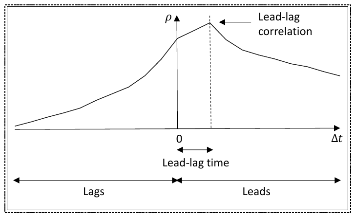
How to read it. The height of the peak is called the lead-lag correlation, its horizontal position the lead-lag time. To the left of zero is the lag side (lags), to the right the lead side (leads).
3.3 The lead-lag ratio
What this is. Formula (6) of the paper, the lead-lag ratio of Huth and Abergel: how much higher the correlation curve is on the lead side than on the lag side.
What each symbol means. The numerator is the sum of squared correlations at all positive shifts (10 points from +10 to +100 ms), the denominator at all negative ones (from −10 to −100 ms). Above one: the shifted instrument leads more often than it follows.
A worked example (our calculation). For the index–IVV pair the correlations on the curve are about 0.193–0.194. Ten squares on each side give a sum of about . LLR = 1.0058 from table 3 means that the sum on the lead side exceeds the sum on the lag side by only 0.58 %.
Why a third quantity is needed. The peak describes one point of the curve. The authors show in a separate diagram a case where the peak sits on the lead side while the whole curve is higher on the lag side.
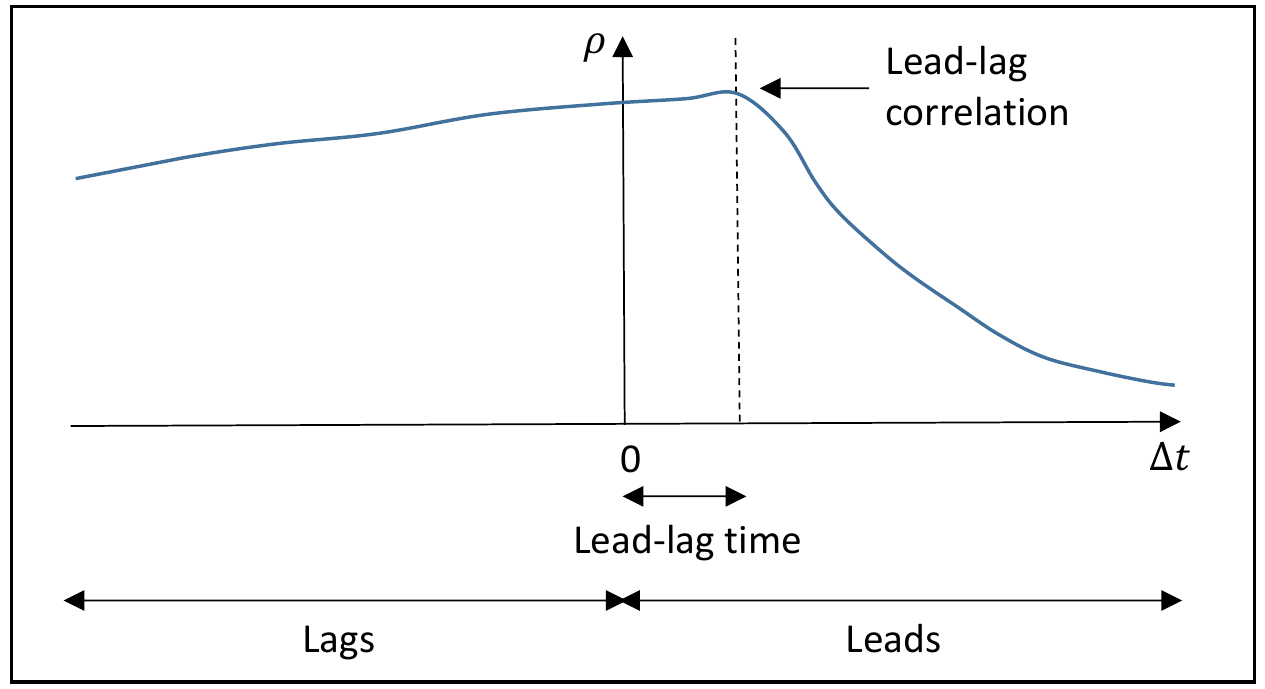
How to read it. The peak of the curve is to the right of zero, on the lead side, so by the peak the shifted instrument leads. But on the left the curve is almost everywhere higher than on the right after the peak, and the LLR will be below one: by the whole curve this instrument rather lags.
The practical takeaway. Both quantities must be reported. The peak and the lead-lag ratio can point in different directions.
4. Data
The S&P 500 index and two ETFs, SPY and IVV, from August 2014 to July 2015, from the Thomson Reuters Tick History database, with timestamps to the millisecond. For the index the values are used, for the ETFs trade prices. Only the regular session from 9:30 to 16:00 is included. Cleaning follows Marshall and coauthors (2013): observations with an absolute log return above 25 % and observations in the first and last five minutes of the session are discarded. In a footnote the authors write that with thresholds of 5, 15, 35 and 45 % the results are the same.
After cleaning (table 1): 17,745,864 index observations, 4,117,085 for SPY and 281,734 for IVV. The median return is zero for all of them, because many trades in a row go at the same price. Average daily volume (table 2): 525 million shares for the index, 29.9 million for SPY, 0.77 million for IVV.
5. Who leads whom
Table 3 of the paper is computed over the whole sample at once, not by day.
| Pair (first is the leader) | Lead-lag correlation | Lead-lag time, ms | LLR |
|---|---|---|---|
| S&P 500 – IVV | 0.1943 | 10 | 1.0058 |
| S&P 500 – SPY | 0.1886 | 30 | 1.0230 |
| IVV – SPY | 0.2370 | 20 | 1.0284 |
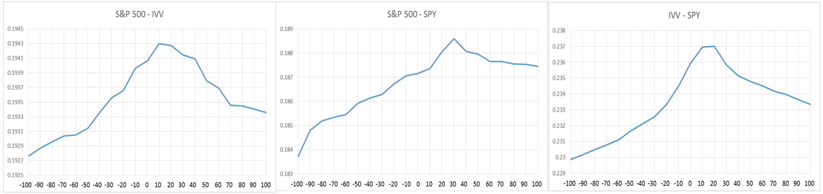
How to read it. Horizontally, the shift of the timestamp of the pair's first instrument in milliseconds; vertically, the correlation. The authors put the curves on three separate charts because on a common one all three would look like straight lines: the correlation range for each pair is very narrow. Note the vertical axes: for the index–IVV pair the whole chart fits between 0.1925 and 0.1945.
What to notice. All three curves peak to the right of zero: the first instrument of the pair leads. From the peak the correlation decreases smoothly in both directions. The ETF–ETF curve is smoother, and the curves with IVV are more symmetric than the index–SPY curve. For the IVV–SPY pair the values at +10 and +20 ms are almost equal.
The practical takeaway. The whole difference between “leads” and “does not lead” here lies in the third digit of the correlation. The measurement requires millions of observations, and its precision is limited by the 10 ms grid step.
The authors' conclusion: the index leads both funds, "so price discovery starts from the index and the ETFs follow" (section 5.1). The correlation of the funds with each other is higher than with the index, and the LLR is slightly above one and highest for the pair of funds.
6. How information arrival affects lead-lag
Information cannot be seen directly, so the authors use the standard proxy: trading volume. The daily volume of each instrument is split along two dimensions.
Block and non-block. Block trades, large by number or value of shares, are usually initiated by institutional participants, according to Madhavan and Sofianos (1998). The authors use them as a proxy for “sophisticated” participants. Non-block volume is the total minus block volume.
Expected and unexpected. Following Bessembinder and Seguin (1993), expected volume for a day equals yesterday's, and unexpected volume is the difference:
What this is. Formulas (8) and (9) of the paper for block volume; for non-block volume (10) and (11) are built the same way.
What each symbol means. : block volume on day . : expected block volume, simply yesterday's. : unexpected block volume, the increase over yesterday. Unexpected volume serves as a proxy for information arrival, expected volume for the usual level of activity.
A worked example (our example). Yesterday SPY's block volume was 5 million shares, today 8 million. Expected 5, unexpected +3 million. If today it is 4 million, unexpected is −1 million.
Each of the three lead-lag measures (correlation, time, LLR) for each day is regressed on four volume components of both instruments in the pair (formula 12 of the paper):
What each symbol means. : the lead-lag measure on day . : four volume components (expected and unexpected, block and non-block) in millions of shares. , : the coefficients being estimated. : the residual. For the pair of two funds the index volume is also added to the regression (formula 13), 12 variables in all.
Results for LLR, the strength of leadership (table 4, panel C). This is the paper's main result.
- Index–IVV: the leader's (index's) unexpected volume strengthens leadership, coefficients +0.00196 for block and +0.00045 for non-block, both significant at 1 %.
- IVV–SPY: the lagger's (SPY's) unexpected volume weakens leadership, −0.00246 for block (1 %) and −0.00227 for non-block (5 %).
- Index–SPY: not a single significant volume coefficient.
Results for the lead-lag correlation (panel A). Here the sign depends on the pair. In the index–IVV pair a rise in the leader's unexpected volume lowers the correlation (−0.00073 for block, 5 %), while a rise in the lagger's volume raises it (+0.05245 for block, 5 %, and +0.03540 for non-block, 10 %). In the other two pairs it is the other way round: in the IVV–SPY pair unexpected block volume of the leader IVV raises the correlation (+0.04518, 5 %), and unexpected volume of the lagger SPY lowers it (−0.00118 for block, 5 %, −0.00112 for non-block, 10 %). The authors put it exactly this way: the effect on correlation of the leader and of the lagger is opposite, but its direction differs between pairs.
Results for the lead-lag time (panel B). Not a single volume coefficient is significant. The intercepts are 9.0 ms, 23.9 ms and 15.4 ms.
The adjusted of the regressions is 0.209 to 0.275 for correlation, 0.113 to 0.151 for time, 0.139 to 0.252 for LLR.
Size of the effects (table 5). The authors convert the significant results into the change in the measure for a one standard deviation rise in volume:
| Pair | Whose volume | Correlation, abs. | Correlation, rel. | LLR, abs. | LLR, rel. |
|---|---|---|---|---|---|
| Index – IVV | leader | −0.0477 | −24.57 % | +0.1453 | +14.45 % |
| Index – IVV | lagger | +0.0545 | +28.03 % | −0.0267 | −2.66 % |
| IVV – SPY | leader | +0.0429 | +18.08 % | +0.0395 | +3.84 % |
| IVV – SPY | lagger | −0.0553 | −23.35 % | −0.0800 | −7.78 % |
How to read the relative numbers. They are given as percentages of the overall level from table 3. For LLR this level is about 1.0, while the asymmetry itself, the excess over one, is 0.006–0.028. So a shift of the LLR by 0.1453 on a given day is much larger than the entire asymmetry over the sample: from day to day leadership wanders far more than the yearly figure suggests (our comment).
The authors conclude that in all pairs the laggers affect correlation more strongly than the leaders, and that index volume affects LLR the most. And a separate conclusion: block volume matters more significantly than non-block volume, that is, sophisticated participants determine lead-lag more strongly.
7. The trading test
Section 5.1 after figure 5 contains one sentence about trading. The authors applied the strategy of Alsayed and McGroarty (2014), trading the lagger in the direction of the leader's previous price change: "However, the strategy is not profitable, which is consistent with Brooks et al. (2001), who find that although the lead-lag effect can be used to produce accurate forecasts, trading these forecasts does not yield favourable returns."
What can and cannot be taken from this. What can: the simplest strategy on a 10–30 ms lead for these instruments, according to the authors, did not make money. What cannot: why exactly. The paper has no return, no number of trades, no accounting for costs, no execution latency, no test period. So it is unknown whether the result was eaten by commissions, the spread, or the fact that 10 ms is less than the real order submission latency.
8. What is shaky in the paper
The authors' own caveats
The wording is cautious. In the abstract leadership "may strengthen or weaken depending on whether the leading or lagging instrument responds to that information", and the effect on correlation likewise "may also have opposite effects". Priority is claimed with the caveat "To our knowledge".
Volume is only a proxy for information. The authors rely on the literature where volume is used as a proxy for the rate of information arrival, and block trades as a proxy for institutional participants. The paper has no direct check that unexpected volume is related to news.
What a reading shows
A trading test without numbers. See section 7. This is the only place in the paper that touches money, and it cannot be verified.
Expected volume equals yesterday's. This is the simplest model of expectation. Regular volume spikes (expirations, index rebalancing, month end, Mondays) will fall into “unexpected” volume and will look like information arrival.
Index volume is not described. The index has no trades of its own, yet table 2 gives it 525 million shares per day, and the regressions include block and non-block index volume. How these numbers were obtained (from the index components or otherwise) and what counts as a block trade for the index, the paper does not say.
Significance is moderate, observations are few. The regressions are daily on one year of data (about 250 trading days; the paper does not give the exact number of days), with 8 or 12 variables. Most significant volume coefficients are at the 5 or 10 % level; at 1 % three coefficients in the LLR panel are significant. There is no correction for testing many coefficients across nine regressions.
Volume and lead-lag on the same day. Volume and the lead-lag measures are taken for one and the same day. The regression shows an association but does not say that volume causes the change in leadership rather than the reverse. This is a limitation of the design, not an error; the authors phrase the conclusion as an effect.
The direction of the effect on correlation is not the same across pairs. In the index–IVV pair the leader's volume lowers correlation; in the IVV–SPY pair it raises it. The authors note this but do not explain it.
A 10 ms grid is coarse for such lags. A lead-lag time of 10 ms for the index–IVV pair is the first step of the grid, and for the IVV–SPY pair the correlations at +10 and +20 ms are almost equal. The method cannot distinguish faster effects.
The less liquid fund leads the more liquid one. IVV has 15 times fewer observations and almost 40 times less volume than SPY, yet by table 3 it leads SPY by 20 ms. The paper does not discuss this. Our remark.
Two figures numbered 5. In the authors' version the diagram explaining LLR (page 12) and the real correlation curves (page 17) are both captioned as figure 5. This does not affect the conclusions, but when referring to the figures it is worth giving the page.
The data period is old. August 2014 – July 2015. Market infrastructure has changed since then, and the absolute lags most likely have too.
9. What follows in practice
Compute the correlation of non-synchronous series over overlapping intervals. The Hayashi–Yoshida estimator does not require alignment to a grid and does not invent points. It suits any pair with its own trade rhythm: different exchanges, spot and futures, a fund and its basket.
Describe lead-lag with three numbers. The position of the peak, its height and the LLR over the whole curve. A peak on one side with the LLR on the other means that the “leader” leads only on a narrow range of shifts.
A correlation without a sampling frequency is not a number. 99.9 % on daily data and about 20 % on ticks for one and the same pair. Decisions made on daily correlations do not carry over to intraday scales.
Compare the lead-lag time with your own latency before any backtest. If the leader leads by 10–30 ms and the path from receiving data to the order reaching the exchange is longer, the strategy is closed. According to the paper the lead-lag time does not depend on daily volume, so it is reasonable to measure it separately and review it when the infrastructure changes (our conclusion from panel B).
The strength of leadership changes from day to day. On days when the lagging instrument trades unusually heavily, leadership is weaker. This is a testable hypothesis for a signal filter, but in the paper it is confirmed on one year of data and at significance levels of 1–5 %.
Statistical distinguishability is not profit. An LLR of 1.02 is distinguishable from one on millions of observations, and the simplest strategy built on it is, according to the authors, unprofitable.
10. Testable ideas
| No. | Idea | Type | Where to compute |
|---|---|---|---|
| 1 | Implement the Hayashi–Yoshida correlation over overlapping intervals and compare it with the correlation over aligned bars on your own pairs with non-synchronous trades | diagnostic | Python |
| 2 | Build the correlation curve by shift (for example, from −500 to +500 ms) for your own pairs of venues or instruments and report three numbers: the peak, its position and the LLR | diagnostic | Python |
| 3 | Compare the measured lead-lag time with your own latency from receiving data to the order reaching the exchange; if yours is longer, close the idea before the backtest | acceptance metric | any |
| 4 | Report the LLR next to the peak position and flag separately the pairs where the peak and the LLR point in different directions | audit | Python |
| 5 | Plot the pair's correlation as a function of sampling frequency (tick, 1 s, 10 s, 1 min, 5 min, hour, day) to see from which scale correlation estimates are applicable at all | diagnostic | Python |
| 6 | Compute the LLR and the lead-lag time for each day and check whether leadership weakens on days with abnormal volume of the lagger, as in the IVV–SPY pair | diagnostic | Python |
| 7 | Replace “expected volume = yesterday's” with a 20-day average adjusted for day of week and expirations, and check whether the volume effects survive | audit | Python |
| 8 | Split the flow into large and small trades and check which part is more strongly related to the strength of leadership | diagnostic | Python |
| 9 | Repeat the simplest strategy “trade the lagger in the direction of the leader's last move” with explicit costs and execution latency, to get the numbers the paper does not have | acceptance metric | backtester |