How to read this walk-through. This is not a paper about markets but a dissertation on systems programming. A trader needs it for one reason: a trading system must record what it saw and what it did, otherwise a live session cannot be reconstructed, and writing to the log on the hot path can cost more than the decision itself. The work shows how to make logging almost free and what is paid for it. The main conclusion is in the section “The method in one line”. The part most transferable to trading code is gathered in section 4 on the buffer design: these techniques fit any queue between threads, from market data to the strategy and from the strategy to execution. The chapters on C++17 metaprogramming and on compression (4, 6, 8) are summarized briefly and can be skipped.
1. Why a trader needs a paper on logging
A log is lines of the form “time, file, line of code, level, message” that a program writes while it runs. They are used later to reconstruct what happened: why an order went out late, why the strategy did not enter, where the system got a stale quote. The more events are recorded, the more useful the log.
The author starts from the fact that logging has become expensive relative to the programs themselves. Formatting one line in a typical system takes 0.5–1 µs, which is 1,000–2,000 processor cycles. One message weighs 50–100 bytes, so a disk at 250 MB/s accepts only a few million messages per second. For servers that respond in 1–2 µs, one log line can double the response time. The author writes that at Google and VMware code reviews include arguments over whether to keep a log line or remove it for speed, and sums up: "Logging itself is expensive, but lacking proper logging is very expensive." (chapter 1).
For a trading system the situation is the same, only the scale is harsher: if a signal lives for tens of milliseconds and the record “sent the order” costs a microsecond on the hot path, logging starts to compete with the decision itself. The usual way out, which programmers outside trading use too, is to write less: raise the severity threshold, skip messages selectively, strip out “unnecessary” lines. The author notes that all these techniques buy speed at the cost of visibility.
2. The method in one line
On the hot path, write into memory only what changes from call to call (the timestamp, the message number, the argument values), in binary form; write everything constant to the file once; assemble the human-readable text in a separate program after the run.
The idea rests on two observations by the author (section 2.3). First: most messages are never read by a human; other programs consume them, and a human looks at a small fraction of the log while debugging. Second: in a line like Creating table 'orders' with id 11 only the time, the thread number, the table name and the number 11 change. The file name, line number, level and message template are known at compile time and repeat in every call.
Hence the three parts of the system (figure 3.1 of the paper):
- at compile time a separate component finds all log calls, extracts their constant part into a dictionary and generates for each call its own write function
record()and compression functioncompress(), with no parsing of the format string at runtime; - at runtime the thread copies the timestamp, message number and arguments into its own buffer in memory and returns immediately; a background thread picks up the data, compresses it and writes it to disk;
- after the run a separate program joins the dictionary with the binary records and prints ordinary text, or hands the records to an analysis program without turning them into text.
The system takes the timestamp straight from the processor's cycle counter (Intel TSC) and does not convert it to hours and minutes at runtime: the mapping between the counter and wall-clock time is written in the file header, and the postprocessing program does the conversion (section 5.3).
3. Where the nanoseconds are won
The author names four techniques the speed rests on (section 3.1 and chapter 12).
Deferred formatting. The most expensive step is removed from the run entirely: the format string is not parsed and numbers are not converted to text.
Separating the constant from the changing. The constant part is written to the file once; after that each call writes only the message number and the arguments. For a fully constant message this is 3–4 bytes instead of 41–90 bytes in other systems (section 9.1.3).
Pre-generated logic. Parsing a format string at runtime requires many branches, and they do not get along well with the processor's out-of-order execution and branch prediction. The functions generated for each call run as straight-line code with almost no branches.
Light compression. Once the constant part is removed, the log holds mostly integers, and small ones: the message number usually fits in 1–2 bytes although 4 are allocated to it, and a timestamp difference under 15 ms fits in 3 bytes out of 8. So instead of dictionary algorithms like gzip the author drops the leading zero bytes and writes a short length marker (chapter 8). Strings and floating-point numbers are not compressed this way.
What a hot path is. The stretch of code that runs on every event and whose speed determines the system's reaction time. In a trading system it is the path from the arrival of market data to sending the order. Everything that can be done later or in another thread is moved off the hot path.
4. The staging buffer: chapter 7 step by step
Chapter 7 is the most useful one for anyone writing multithreaded trading code. The author starts from the simplest solution and improves it step by step, from latencies of micro- and milliseconds down to single nanoseconds.
Step 0: a shared queue with a lock. All threads write into one queue protected by one lock (mutex). There is one advantage: the order of messages comes out by itself. There are three drawbacks. All threads line up behind each other. The background thread cannot read while someone is writing. And the lock itself is expensive: a write in NanoLog takes about seven nanoseconds, while "a lock operation can take several times longer as it requires explicit and excessive cache synchronization" (section 7.2). Worse, some lock implementations put the waiting thread to sleep, and then an operation of nanoseconds stretches to milliseconds until the operating system returns the thread to work.
Step 1: each thread has its own buffer. The threads that write the log stop running into each other. The price is twofold: a memory allocation when the thread is created (no more than once per thread) and the loss of global order. Within one buffer messages are ordered by time; across buffers they are not. Sorting moves to postprocessing. The allocation can be done in advance with a separate call so that it does not coincide with a time-critical section.
Step 2: lock-free, one writer per variable. The buffer is a ring with two markers: producerPos, where the application thread writes, and consumerPos, where the background thread reads. Only the writing thread changes the first, only the background thread changes the second, and either can read both.
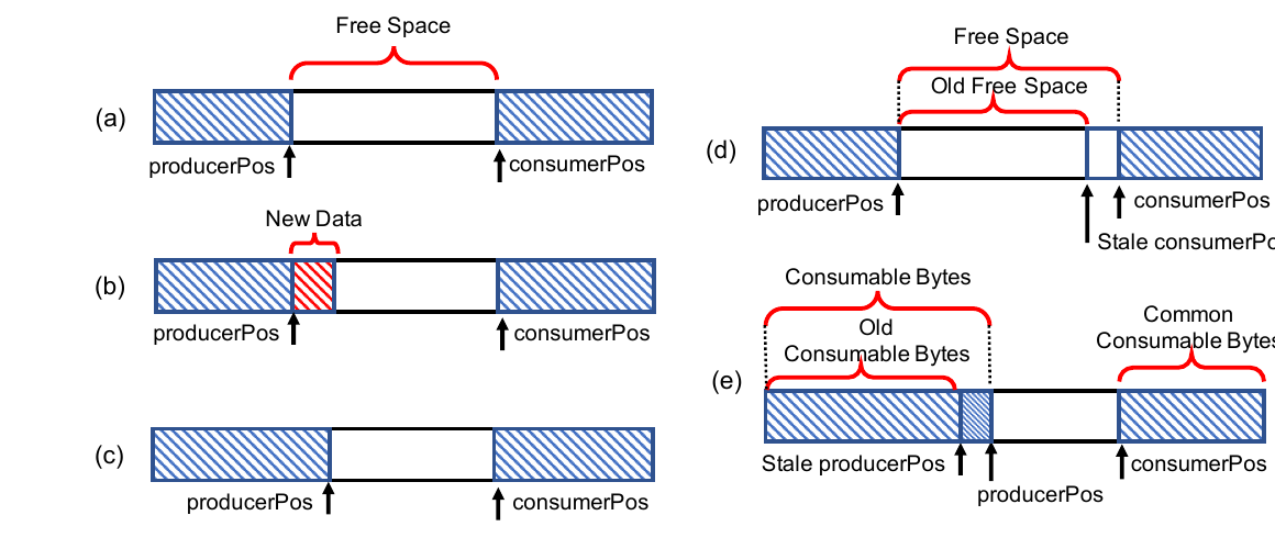
How to read it. Hatched regions hold data, white ones are free. Parts (a)–(c) show a write: (a) free space is computed as the difference between the reader's position and the writer's position; (b) if there is enough room, the new data are copied to the writer's position; (c) the writer's position moves past the new data.
What to notice. Parts (d) and (e) explain why no lock is needed. In (d) the writer uses a stale value of the reader's position (
Stale consumerPos). The reader may have moved on in the meantime and freed more room, so the “old free space” (Old Free Space) is always smaller than the real one and lies entirely within it. In (e) the same holds from the other side: the reader, using a stale writer position, sees less ready data than there is.The practical takeaway. If the error from a stale value always goes in the cautious direction, no synchronization is needed: in the worst case the thread needlessly declines to write or reads the data on the next pass, but it never overwrites unread data.
The author puts it this way: free space can only grow over time, so "using an old value would only at worse underestimate the free space" (section 7.4). Two conditions are mandatory here, and they are easy to miss when carrying the technique into your own code. First, the order of memory operations. The writer first puts down the data and issues a store fence, and only then moves its position; the reader first finishes reading the data with a load fence, and only then moves its own. Second, in a footnote the author states the assumption "Individual reads and writes to single-word values are assumed to be atomic." (section 7.4). There is also a third detail: when a record does not fit at the end of the ring, the writer marks the end of the occupied region with a separate pointer and wraps to the start; this pointer is also written before the position moves.
If there is not enough room, the write function returns an error and retries. In other words, when the buffer overflows the writing thread waits. This is an important detail for a trading system; we return to it in section 6.
Step 3: remember the other side's position. The lock-free scheme is still expensive under load: to compute free space, on every write the writer reads a position that another thread on another core has just changed. Such a read misses the cache, and "This cache miss can slow the operation by tens of nanoseconds" (section 7.5), that is, several times more than the write itself. If both threads run in lockstep, the miss happens on every operation.
The solution: each thread keeps its own counter of free (or ready-to-read) space, subtracts from it on every operation and goes to read the other side's position only when the counter runs out. This is safe for the same reason as step 2: the remembered value is equivalent to a deliberately “frozen” stale position, and a stale position never overstates free space.
How it works in numbers (our example; the paper gives no numbers). A 1 MB buffer, an average record of 100 bytes. Without remembering, the writer reads the reader's position on each of the 10,000 records that fit into the buffer: 10,000 expensive reads. With remembering, it learns once that 500 KB are free, and for the next roughly 5,000 records it does not touch the other thread's memory at all. The number of expensive accesses falls by a factor of thousands, provided the reader keeps freeing room.
Step 4: put the variables on different cache lines. Even after step 3 the writer's and the reader's counters may end up on the same cache line. Then a write to one's own counter evicts the neighboring counter of the other thread from the cache, although logically they are independent. This is false sharing. NanoLog inserts an empty array the size of a cache line between the writer's variables and the reader's variables.
What a cache line and false sharing are. The processor moves memory between cores not byte by byte but in fixed-length blocks; on common x86 processors this is 64 bytes (the size is ours; the paper does not name it). If core A has changed a variable, the copy of the whole block in core B's cache is considered stale, and on the next access B goes for a fresh copy. When two independent variables written by different threads sit in one block, they get in each other's way with no logical connection at all. This cannot be seen by reading the code.
Step 5: polling instead of signaling. The classic way to tell the background thread that data have appeared is a condition variable (condition_variable::notify()). The author measured it: "The notify operation takes on the order of 14 nanoseconds in my measurements" (section 7.7), twice the target of 7 ns for the whole write. So the application thread signals no one, and the background thread itself walks the buffers in a loop. The flip side: between polling rounds the background thread sleeps, and this shows up in the latency tail (section 5).
Step 6: the metadata of all buffers in a row. At first each buffer's metadata (positions, counters, separators) sat next to its storage, and the metadata of neighboring buffers ended up in memory a storage size apart. The processor's prefetcher did not guess the next address. When the metadata of all buffers were gathered into one contiguous region, polling each buffer became cheaper by roughly one cache miss (section 7.8).
The chapter's result in the author's words: the buffers operate "in the range of single digit nanoseconds vs. the micro- to milliseconds incurred by a centralized, monitor-style queue" (section 7.9).
5. What the measurements showed
The test machine (table 9.1): a four-core Xeon X3470 at 2.93 GHz, 24 GB of memory, a Samsung 850 PRO SSD with a measured speed of about 250 MB/s on large writes, Debian 8.3 with Linux kernel 3.16.7. The comparison covered Log4j2, spdlog, glog, Boost Log and Event Tracing for Windows (ETW) on six messages from the open-source RAMCloud storage system: from a fully constant string to a string with long variable text.
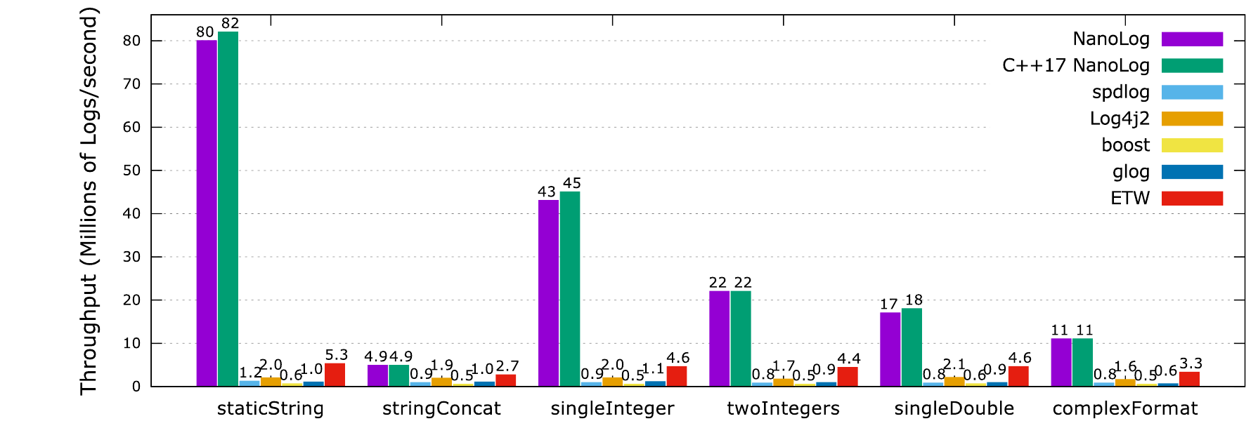
How to read it. Horizontally, the six benchmark messages; vertically, millions of messages per second. Each group has seven bars: two versions of NanoLog and five other systems. “NanoLog” here is the preprocessor version, “C++17 NanoLog” is the version built on C++17 templates. The number of threads varied from 1 to 16 and the best result is shown; for all systems except Log4j2 the measurement includes flushing to disk.
What to notice. On the constant string (staticString) NanoLog delivers 80–82 million messages per second against 0.6–5.3 million for the others. On the string with long variable text (stringConcat) the gap almost disappears: 4.9 million against 0.5–2.7 million. NanoLog does not compress strings and writes them in full, so the more text a message holds, the smaller its advantage.
The practical takeaway. NanoLog's gain is a gain in bytes per message. The log of a trading system, where messages are mostly numbers (prices, volumes, identifiers), is closer to the right half of the chart, to messages with integers and floating-point numbers, where NanoLog delivers 11–45 million.
For the latency of a single call (table 9.4: one thread, 100,000 calls in a row with a 600 ns pause between them) NanoLog's median is 7–8 ns, and the 99.9th percentile is 27 to 37 ns. ETW has a median of 180–242 ns, Log4j2 146–230 ns, spdlog 230–1,234 ns, glog 1,201–2,570 ns, Boost 1,619–4,175 ns. The author sums this up as: NanoLog's call latency is 18–500 times lower than that of the other systems.
Embedding in a real application. The author embedded NanoLog and spdlog into the RAMCloud key-value store, turned on all verbose messages and added continuous performance measurements, 11–33 log calls per read or write request in total (table 9.6). With NanoLog the median read latency rose by 3 %, write latency by 3–4 %, write throughput fell by 2 %, read throughput by 19 % (RAMCloud's dispatch thread is already the bottleneck on reads). With spdlog latencies grew 1.6 times, read throughput fell to 12 % of the original, and with RAMCloud's built-in log to 7 %.
From these numbers the author estimates the price of one call in real work:
What this is. The price of one log call inside a real application, not in a microbenchmark.
What each number means. 5.33 µs: the median read latency in RAMCloud with the NanoLog log. 5.19 µs: the same without the log. 8: how many of the enabled messages lie on the critical path of one read.
Step by step. Subtract one time from the other: the log added 0.14 µs. Divide by 8 calls: 0.0175 µs per call, that is, 17.5 ns. For writes (27 calls on the critical path) the author gets 17.7 ns.
Why this matters. This is 2–2.5 times more than the 7–8 ns of the microbenchmark. The author supposes that the difference comes from cache misses on the buffers and says directly that they could not check this more deeply. For spdlog the same calculation gives about 380 ns, close to the microbenchmark.
The RAMCloud build with the preprocessor version became 17 % longer and the binary 16 % larger; with the C++17 version the build is 2 % longer and the binary 19 % larger.
Where the bottleneck is. Figure 9.5 shows what exactly limits throughput.
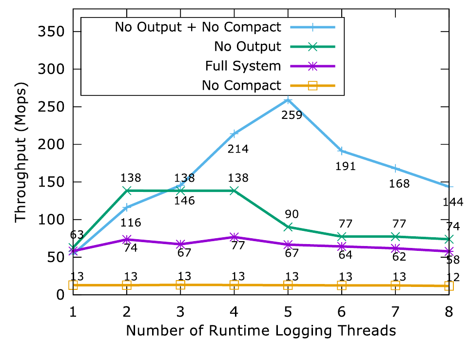
How to read it. Horizontally, the number of threads writing the log (from 1 to 8); vertically, millions of messages per second. Full System is normal operation. No Output sends the log to
/dev/null, that is, removes the disk. No Compact turns compression off. No Output + No Compact removes both.What to notice. Without compression throughput falls to 13 million: a message weighs about 16 bytes instead of 3–4, and the disk cannot keep up. Without the disk it rises to 138 million, and compression becomes the bottleneck. Without either it reaches 259 million at five threads and then falls: the machine has 4 physical cores, and the application threads start taking processor time from the background thread.
The practical takeaway. On ordinary hardware the limit is set by the volume of bytes going to disk, not by the write code. Hence the value of compression on the hot path, which at first sight looks like extra work.
The author shows why compression cannot simply be dropped with a faster disk:
Step by step. 138 million messages per second (what the system delivers without the disk) times 16 bytes of an uncompressed message: about 2.2 billion bytes per second. That is the disk needed to sustain the same speed without compression, not a disk twice as fast as the test machine's.
The latency tail and buffer size. Figure 9.6 is for those who think about the worst case, not the median.
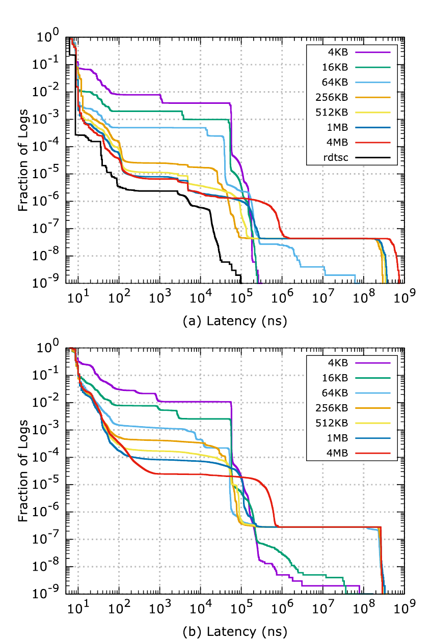
How to read it. This is the complementary cumulative distribution function (CCDF): a point (x, y) means that a fraction y of all calls took at least x nanoseconds. Both axes are logarithmic. The upper panel is for the constant string, the lower one for a complex message. Each curve is a billion calls in a row with no pauses from one thread, so the log is written faster than the disk can keep up by design. The black rdtsc line on the upper panel is a billion reads of the cycle counter in a row, the lower bound of what is possible on this machine at all.
What to notice. Regardless of buffer size, 90 % of calls are faster than 10 ns. The larger the buffer, the larger the share of fast calls: about 90 % at 4 KB, 99.8 % at 512 KB; beyond 512 KB the gain barely grows. Then come two steps. Around 50 µs: the background thread sleeps between polling rounds, and a small buffer has time to fill. Around 100+ ms: the 64 MB output buffer has filled, and everyone waits for the disk.
An unexpected consequence. The slowest write is worse with a large buffer. At 4 KB the worst call takes tens of microseconds, at 4 MB hundreds of milliseconds. The author explains: a small buffer stalls the writing thread often and briefly, and the disk keeps up; a large one accumulates more and then waits for the disk longer. In the author's words,
"the more frequent the stalls, the better the worst-case performance"(section 9.6).
By default NanoLog uses a 1 MB buffer, beyond which the share of fast calls barely grows. The author immediately notes that the experiment is artificial: the application only writes the log and does nothing between calls. At a reasonable pace, for example one message per 1,000 ns, the author expects a noticeably better tail closer to the rdtsc line, but even then latencies of about 100 µs are possible for reasons outside the application.
The rest of chapter 9 in brief. The postprocessing program is single-threaded and converts about 0.5 million messages per second to text; almost all the time goes to formatting the date and context, about 2 µs per message. Sorting 4,096 threads lowers its speed by about 10 %. Aggregation (minimum, mean, maximum over one message) directly over the binary log costs 35–44 ns per message against 350+ ns for C++, awk and Python over a text log; the binary file weighed about 747 MB against 7.6 GB of text, and the difference is almost entirely explained by the volume read from disk.
6. What is shaky in the paper
The author's own caveats
The microbenchmarks describe the best case. About the latency table the author writes that the results "may represent an unrealistic, best-case performance for all logging systems" (section 9.1.4): the application in the test only writes the log, does not pollute the cache in any way and does not compete for the disk and the processor. The RAMCloud embedding confirms this: 17.5 ns instead of 7–8.
The latency tail experiment is artificial. "this benchmark is a bit unrealistic/contrived" (section 9.6). It shows behavior under overflow, not under normal load.
On overflow the writing thread waits. NanoLog guarantees that no message is lost and pays for this with blocking: "NanoLog can block, but will never miss any critical events" (section 11.5). Tracing systems like KUTrace do the opposite: they overwrite old events and never slow the application down. The author openly admits that NanoLog's latency spread is larger than theirs because of this, and describes how to bring NanoLog closer to a tracer: disable the background thread, flush to disk after the observation window, enlarge the buffer, limit the number of arguments.
The order of events is restored afterwards, and there is a rare case where this may fail. Postprocessing holds two output rounds and merges them by timestamp. If a thread read the cycle counter, was preempted by the scheduler and did not finish writing its arguments for longer than two rounds, its message will land in the file after later ones. The author put a check on this case and writes that it never fired, although thousands of threads were running on 4–8 cores; the GitHub version keeps three rounds just in case (section 6.1.4).
Four fundamental limitations (section 10.2). The system adds a separate build step and a separate postprocessing program, that is, new points of failure. If a human needs the log as text anyway, more resources are spent in total than with an ordinary library, and the author states the condition of applicability: "NanoLog only makes sense in situations where runtime performance is paramount". Only the printf style with a constant format string works; dynamic format strings and printing data structures are not supported. And finally, "NanoLog is not a silver bullet to application visibility": what to log and where is still the developer's decision, and unnecessary messages make analysis harder.
Explanations the author did not check. Why ETW is slower with a similar design (ETW is closed, and a deeper measurement was not possible), why a call in RAMCloud costs more than in the microbenchmark, why the gain from the buffer stops growing after 512 KB, why compression is sometimes faster than a plain memory copy. Everywhere the text says “I suspect” or plainly “did not check”.
The system's future. In the conclusion the author does not expect the prototype to become a standard: "I don't envision that the NanoLog system will become a staple of logging anytime soon" (section 12.1). The author counts on the techniques being carried over into other systems.
What a reading shows
All measurements were made by the author on their own system. The competitors were configured as the author describes (spdlog with a buffer of 8,192 entries, glog with a 30-second buffer, Log4j2 with asynchronous loggers and the LMAX Disruptor), and the work contains no independent replication. spdlog was chosen, in the author's words, as the first search result for “Fast C++ Logger”. This does not make the comparison unfair, but it means the competitors could have been configured differently.
The hardware is old for 2020. A four-core Xeon and a SATA SSD at 250 MB/s. The absolute numbers on a modern server with an NVMe disk will be different; the author shows (figure 9.5) that with a faster disk compression becomes the bottleneck.
Different numbers in different places describe different messages, not a contradiction. The abstract has "typical log invocation overhead of 8 nanoseconds" and up to 82 million messages per second, the section “Industrial Response To NanoLog” before the table of contents has "median invocation latency of 7-19 nanoseconds", and chapter 1 has about 80 million. 82 million is the C++17 version on the constant string, 80 million the preprocessor version. Readers should take numbers from table 9.4 and figure 9.2 together with the message type.
A direct port to Python is impossible. This is our remark, not the author's: the techniques of chapter 7 rely on the C++ memory model and on fences, which an interpreter with a global lock does not have in the same form. They apply to parts of the system written in C++ or Rust.
7. What follows in practice
Logging on the hot path is possible if you do not format. Write a binary record of minimal size with a timestamp from the cycle counter, and turn it into text in another process, on another core or another machine. This removes the choice between “write a log” and “be fast”, which the author considers a false one.
The single-writer rule instead of a lock. For any shared structure check two things: each variable has exactly one thread that writes it, and a stale value errs in the safe direction. If both conditions hold, the lock can be removed, but only together with correct memory fences.
Do not read the other thread's variable on every iteration. Remember the last value and reread it when the margin runs out. This is a cheap change with an effect on the number of cache misses.
Check the field layout in structures touched by different threads. False sharing is not visible in the code and is not caught by a profiler that shows time per function.
Decide in advance what to do on overflow. Waiting (like NanoLog) means risking an order delay of hundreds of milliseconds in the worst case; dropping (like tracers) means losing events at the most interesting moment. Buffer size shifts this choice: a large buffer makes rare stalls longer, a small one makes them more frequent and shorter.
Measure the tail, not the average. A median of 7 ns says nothing about a hundred-millisecond call once in a billion. A chart like figure 9.6 shows this at once.
The order of events is a design decision with a price. A per-thread buffer is faster than a shared queue, but it requires timestamps in every record and sorting at analysis time. For a log used to reconstruct the sequence of trading decisions, this has to be decided explicitly.
8. Testable ideas
| No. | Idea | Type | Where to compute |
|---|---|---|---|
| 1 | Measure the price of one log call on your system's hot path at the median and the 99.9th percentile, separately in a microbenchmark and under real load (following the 17.5 ns calculation from RAMCloud) | diagnostic | any |
| 2 | Move the hot-path log to binary recording of arguments with formatting in a separate process, and compare the latency from data arrival to order submission before and after | design change | any |
| 3 | Go through all inter-thread structures: each variable has one writer, a stale value errs in the safe direction, memory fences come before the position moves | audit | any |
| 4 | Replace reading the other thread's position on every iteration with a remembered free-space counter and compare latency under load | design change | any |
| 5 | Check the field layout in shared structures and put fields of different writers on different cache lines; measure the difference | audit | any |
| 6 | Report system latency as a complementary distribution function down to the 10⁻⁶ level and below, not as an average | acceptance metric | Python |
| 7 | Run a burst of events faster than the disk can keep up with, at different buffer sizes, and choose the size by the worst call, not the median | diagnostic | any |
| 8 | During postprocessing, check that messages from different threads go in non-decreasing timestamp order after the merge, and count the violations | audit | Python |
| 9 | Replace the signal to the background thread (condition variable) with polling and compare write latency and core load | design change | any |