How to read this walk-through. The paper's main result fits into two formulas, which are in the section “The method in one line”: where to put the center of the quotes and how wide to make the spread. The section on simulations shows what this gives in practice, and it is worth reading in full. The derivation via the Bellman equation can be skipped. Everything the model leaves out is collected in the section “What is shaky in the paper”.
1. How the model's world is set up
A market maker keeps two limit orders in the limit order book: a buy order slightly below the mid-price and a sell order slightly above it. The income comes from the difference. The authors single out two risks the market maker faces. Inventory risk: while a position has built up, the price can move against it. Transaction risk: it is unknown when the orders will be filled, or whether they will be filled at all. The classical literature names a third risk as well, the informed counterparty, but the authors state at the outset that they deal only with the first: "we will focus on the inventory effect" (section 1).
What the model consists of:
- the mid-price moves as a random walk without drift and with constant volatility: ;
- the agent places a buy order at distance below the mid and a sell order at distance above it;
- market orders arrive at random, as a Poisson process, and fill the agent's orders one share at a time;
- is the agent's inventory: plus means long, minus means short;
- is the end of the session, at which the result is evaluated.
What a Poisson process is. A model of events that arrive independently of one another at a known average rate. Example: calls to a call center, 10 an hour on average, but the moments of the calls are random. This is how market orders arrive here and hit the agent's orders.
What is. An increment of a Wiener process, that is, a random push with zero mean. Over a time step the price changes by a random amount with standard deviation .
Why an arithmetic walk rather than the usual geometric one, the authors explain in footnote 1: this keeps expected utility bounded. The appendix has a version with a geometric walk and a “mean minus variance” objective, and the authors write that the substance of the results is preserved.
2. The method in one line
Compute the agent's personal price, shifted against accumulated inventory, and place around it a spread whose width is the sum of a charge for inventory risk and a charge for liquidity.
The first step, the reservation (indifference) price:
What this is. The agent's personal valuation: the price at which the agent is indifferent between holding the position and not holding it. The agent places orders around it, not around the mid-price. The authors stress that this is a subjective valuation, not a trade price:
"We stress that this is a subjective valuation from the point of view of the agent and does not reflect a price at which trading should occur"(section 2.2).What each symbol means.
- : the mid-price, halfway between the best bid and the best ask.
- : current inventory in shares, signed.
- (“gamma”): risk aversion. The larger it is, the more the agent fears fluctuations.
- (“sigma squared”): price variance per unit of time.
- : how much time is left until the end of the session.
Step by step. Multiply inventory, gamma, variance and the remaining time. Subtract the result from the mid-price.
A worked example on the paper's simulation parameters (, , that is, , ):
- inventory : zero shift, the reservation price equals the mid;
- inventory at the start of the session: . With the mid at 100 the reservation price is 98, and both orders move down: the agent is willing to sell below the market and does not want to buy more;
- the same inventory at : , reservation price 99.8. The price will not move far before the end of the session, and the inventory is no longer so frightening.
Why this matters. This is inventory management itself. There is no forecast of direction here: the rule only decides which side to quote more aggressively, based on what has already accumulated.
The second step, the full spread width around the reservation price:
What this is. The distance between the buy order and the sell order. It is placed symmetrically around the reservation price .
What each symbol means. and (“delta a” and “delta b”): the offsets of the sell and buy orders. : how fast the frequency of fills falls as the quote moves away from the mid (section 3). : the natural logarithm.
Step by step. The first term, gamma times variance times the remaining time, is the charge for the risk of holding inventory. The second: divide gamma by , add one, take the logarithm and multiply by ; this is the charge for liquidity, a trade-off between the income from one trade and the number of trades.
A worked example on the paper's parameters (, , , ): the second term is ; the first at the start of the session is . The spread is about 1.69 at the start of the session and 1.29 toward its end.
Why this matters. Width and center are two independent knobs. Inventory moves the center, while the width does not depend on it:
"The bid-ask spread in (3.13) is independent of the inventory. This follows from our assumption of exponential arrival rates."(section 3.2). With a different shape of the flow of fills this property disappears.
The number 1.29 matches the value in the “Spread” column of table 1, and in the simulation text the authors cite exactly this one: "a bid/ask spread of $1.29 (corresponding to the optimal agent with γ = 0.1)".
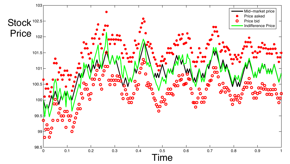
How to read it. Horizontally, time from 0 to 1, one session. The black jagged line is the mid-price, the green line the reservation price (indifference price), the filled red dots the sell orders, the red circles the buy orders.
What to notice. Around the green line is above the black one. By the formula this means : the agent is short. The buy order sits close to the mid, the agent wants to buy back, and, as the authors write, by the inventory returns to zero. Toward the end of the session the green line hugs the black one, and the quotes become almost symmetric.
The practical takeaway. The rule does not guess direction. It tilts the quotes against accumulated inventory and does so more weakly the less time is left.
3. Where the exponential in the flow of fills comes from
Everything the agent knows about the market sits in one function: how often an order placed at distance from the mid gets filled.
What this is. Fill intensity: the average number of fills of an order per unit of time.
What each symbol means. (“lambda”): the intensity. : the intensity at zero offset, an order exactly at the mid. : the decay rate. : an exponential that decreases as the offset grows.
Step by step. Multiply by the offset, raise to minus that power, multiply by .
A worked example on the simulation parameters (, ): at the mid, 140 fills per unit of time; at an offset of 0.5, about 66; at an offset of 1, about 31; at an offset of 2, about 7. Each additional unit of offset divides the flow by roughly 4.5 (); our calculation.
Why this matters. Everything else depends on and : the second term of the spread contains directly. These are characteristics of a specific market at a specific time, and they have to be estimated from your own data.
The authors do not postulate the exponential; they assemble it from two empirical facts of econophysics (section 2.5). The first: market order sizes follow a power law, with density and estimates of for US stocks, 1.4 for NASDAQ and 1.5 for the Paris Bourse. The second: how much a large order moves the price. Here the authors are frank about the disagreement: "There is less consensus on the statistics of the market impact in the econophysics literature." Some find a power-law impact with or 0.76, others get a better fit with a logarithmic one, .
Logarithmic impact together with a power-law tail of sizes gives an exponential with and ; here is the overall frequency of market orders, which the authors suggest estimating as daily volume divided by the average order size. Power-law impact would give a power-law intensity . The authors' conclusion is cautious: "Aggregating these results suggests that λ should decay as an exponential or a power law function." From there on they work with the exponential, because with it the formulas come out in closed form.
4. What the agent maximizes and how the solution is obtained
What this is. The objective function: the expected utility of terminal wealth.
What each symbol means. : cash in the account at the end of the session. : the remaining inventory at the final mid-price. Their sum is terminal wealth. : an exponential utility function; the minus sign makes it increase with wealth . : the average over all scenarios given what is known at time . over : choose the offsets at which this average is largest.
How it reads. The agent cares how the result is obtained: a steady 100 is better than 100 with a large dispersion. Exponential utility makes this difference measurable, and for the derivation it is convenient because the reservation price does not depend on initial wealth. The authors give this property as the reason for the choice (section 2.2).
An example. The authors have three agents: is almost indifferent to risk, is moderately cautious, is very afraid of building up inventory. How they differ is visible in the tables of section 6.
The solution goes through the Hamilton–Jacobi–Bellman equation, the standard tool of dynamic programming, as in the 1981 paper by Ho and Stoll. The full equation is nonlinear and has no closed-form solution. The authors make two simplifications: they expand the solution in powers of inventory up to second order and take a linear approximation of the terms responsible for order arrivals. It is after these simplifications that the reservation price coincides with the price of an agent who does not trade at all and simply holds the inventory until the end of the session, and the spread takes the form from section 2. The authors note that with a quadratic approximation of the flow the sensitivity to inventory would already obey a nonlinear equation. In other words, the formulas of section 2 are approximate and are meant for small inventories.
There are also the exact definitions from which everything grew. The reservation bid price is the price at which the agent is indifferent between buying one more share and not buying it; the reservation ask price is defined the same way. For an agent with no orders they equal , and the reservation price from section 2 is their average.
5. If the session never ends: the infinite horizon
The factor requires a moment at which the inventory has to be valued. In section 2.3 the authors themselves propose a stationary version without an end of session: the agent maximizes discounted utility over an infinite horizon with a parameter .
What this is. The reservation ask price for an agent with no end of session. The reservation bid price is obtained by replacing with .
What each symbol means. (“omega”): the discounting parameter. The formula makes sense for , so the authors read as an upper bound on inventory and propose the natural choice , where is the inventory limit.
Step by step, our example. , , : , . With inventory the denominator is ; for the sell side the numerator is , and ; for the buy side the numerator is , and . Both reservation prices are below the mid: with a long, the agent wants to sell and does not want to buy.
Why this matters. This is the authors' own answer to the question of what to do when the session never ends. Instead of the remaining time, a set inventory limit governs the shift of the quotes.
For this version the authors do not derive the spread and do not run simulations; in section 3 they work with a finite horizon.
6. Simulations: what the inventory adjustment gives
Parameters: , , , , , , . At each step the agent recomputes the offsets, sells one share with probability , buys one with probability , and the mid moves by . The comparison is with a symmetric strategy that has the same spread but whose center is always at the mid-price. There are 1,000 runs for each .
The authors call the choice of the step a subtle point ("In practice, the choice of time step dt is a subtle one."): it must be small enough that more than one order rarely arrives within a step, and larger than the typical interval between ticks, otherwise the orders are recomputed so often that they do not have time to be filled.
| Strategy | Spread | Profit | Std. dev. of profit | Final inventory | Std. dev. of inventory | |
|---|---|---|---|---|---|---|
| 0.1 | inventory | 1.29 | 62.94 | 5.89 | 0.10 | 2.80 |
| 0.1 | symmetric | 1.29 | 67.21 | 13.43 | −0.018 | 8.66 |
| 0.01 | inventory | 1.33 | 66.78 | 8.76 | −0.02 | 4.70 |
| 0.01 | symmetric | 1.33 | 67.36 | 13.40 | −0.31 | 8.65 |
| 0.5 | inventory | 1.15 | 33.92 | 4.72 | −0.02 | 1.88 |
| 0.5 | symmetric | 1.15 | 66.20 | 14.53 | 0.25 | 9.06 |
Tables 1–3 of the paper combined into one.
At the inventory strategy earns 6 % less (62.94 against 67.21), but its profit dispersion is 2.3 times smaller (5.89 against 13.43), and the dispersion of final inventory is 3 times smaller (2.80 against 8.66). Dividing profit by its dispersion gives 10.7 against 5.0 (our calculation from the table; the authors do not compute this ratio).
At the difference almost disappears. The authors write that "in the limit as γ → 0 the two strategies are identical": an agent indifferent to risk has no reason to shift the quotes.
At profit is almost half as large (33.92 against 66.20), with an inventory dispersion of 1.88. The authors describe this agent as a very cautious one that "will go to great lengths to avoid accumulating an inventory".
The authors explain why the symmetric strategy earns more as follows: it is always centered on the mid and therefore gets more fills. The inventory strategy periodically pulls one side away from the market and misses part of the flow.
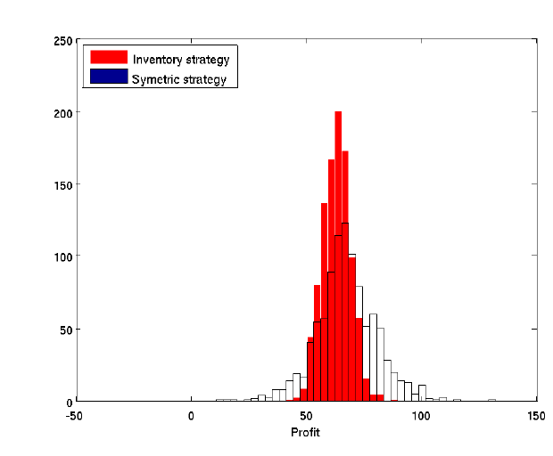
How to read it. Horizontally, profit per session; vertically, the number of runs. Red bars are the inventory strategy (Inventory strategy), white bars with a black outline the symmetric one. The legend assigns dark blue to the symmetric strategy, but on the chart its bars are white.
What to notice. The centers almost coincide, around 60–70. The red distribution is narrow and tall, the white one wide, with tails from 10 to 130.
The practical takeaway. The inventory adjustment barely moves the mean; it compresses the distribution of the outcome.
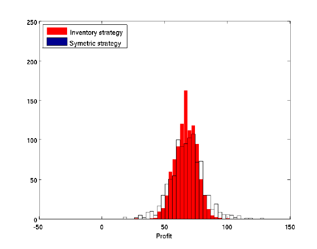
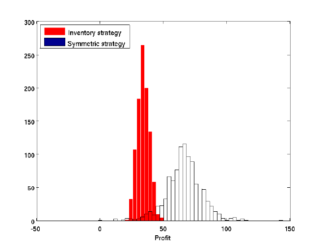
How to read figures 3 and 4. The same axes and colors. Figure 3 shows an agent almost indifferent to risk: the distributions are close, the red one only slightly narrower. Figure 4 shows a very cautious agent: the red distribution is narrow and shifted to the left, to 30–40, while the white one stayed around 65.
The practical takeaway. The parameter works as a “profit versus stability” knob. Three values give three different products, and the choice between them is set by how much dispersion of the outcome is acceptable, not by maximum profit.
7. What is shaky in the paper
The authors' own caveats
The formulas are approximate. The reservation price and the spread from section 2 are obtained by an expansion in inventory and a linear approximation of the order flow (section 3.2). For large inventories and with a quadratic approximation the result would be different, and the authors say so directly.
The shape of the flow is chosen, not established. The authors themselves cite the disagreement on impact and the conclusion “an exponential or a power function”. The independence of the spread from inventory follows specifically from the exponential.
Inventory risk only. The risk of an informed counterparty is set aside from the first page.
The price model is simplified to keep utility bounded (footnote 1), and the version with a geometric walk is given only in the appendix, without simulations.
What stands out on reading
We did not look for discrepancies between the numbers and the text: the paper's numbers and formulas were not recomputed (the “our calculation” mark appears only on our own examples). Below are design limitations that are visible on reading.
No informed flow. The probability that a buy order is filled is the same whether the price is about to fall or to rise. In a real market an order is filled more often when the price moves against it, and this is usually what eats a market maker's income.
No queue. A fill depends only on the distance to the mid, not on the volume standing ahead at the same price level.
Unit size, no fees, rebates or tick size. Every fill is exactly one share.
A finite and known . In a round-the-clock market the factor is undefined. The infinite-horizon version from section 5 exists, but without a spread and without simulations.
Checked with the same model. All 1,000 runs were done in a world where the assumptions hold exactly. There is no empirical check.
The “Spread” column in the tables. For the value 1.29 matches the second term of the spread formula, without the inventory part , which adds another 0.4 at the start of the session. Whether this part is included in the spread of the symmetric strategy, the text does not specify; it says only that the symmetric strategy "uses the same spread as the inventory strategy". How fair the profit comparison is depends on this.
8. What follows in practice
Inventory management and direction forecasting are different layers. The construction contains not a single price forecast. It is convenient to keep the signal part of a bot and its inventory part separate and to test them separately.
The reservation price is one line of code: r = mid - q * gamma * sigma**2 * (T - t). All the difficulty lies in calibrating , and especially and .
and matter more than the formulas. Without your own estimate of the “fill frequency versus offset” relationship, the spread from the formula remains a number from someone else's market. If the relationship is not exponential, the spread-width formula is wrong by construction.
is chosen from the acceptable dispersion, not fitted to profit. On historical data, maximizing profit will almost always give near zero, that is, the symmetric strategy with twice the dispersion.
The “dispersion of final inventory” metric stands on a par with profit in the paper. For any market-making strategy it is a direct sign of whether inventory control works.
For a round-the-clock market it is more honest to start with the infinite-horizon version from section 2.3 of the paper, where the inventory limit is set explicitly, than to plug an arbitrary constant into .
9. Testable ideas
| No. | Idea | Type | Where to compute |
|---|---|---|---|
| 1 | Estimate from your own limit order book the “order offset from the mid → fill frequency” relationship and check whether it is an exponential or a power function; get your own and | diagnostic | Python |
| 2 | Add the quote-center shift as a separate switchable module and compare with the symmetric version on profit, profit dispersion and dispersion of final inventory | design change | backtester |
| 3 | Run a grid of from 0.001 to 1 and plot the “mean profit versus its dispersion” curve; choose the point by the acceptable dispersion | acceptance metric | Python |
| 4 | For a market that never closes, compare three replacements for : a constant, a rolling window, and the infinite-horizon version with an inventory limit | design change | Python |
| 5 | Add informed flow to the simulation: fills happen more often when the price then moves against the order; check whether the advantage of the inventory adjustment survives | diagnostic | Python |
| 6 | Add a queue at each price level to the simulation and see how the optimal offset changes | diagnostic | Python |
| 7 | Check on real fills that the spread width should not depend on inventory; if a dependence appears, the flow of fills is not exponential | audit | Python |
| 8 | Include the dispersion of final inventory per session in the standard report of any market-making strategy, next to profit | acceptance metric | backtester |