How to read this walk-through. The paper is short, and the main thing in it is one formula: the deflated Sharpe ratio. Without formulas, the conclusion is this: before celebrating the Sharpe of the best variant, compare it not with zero but with the Sharpe that the best of variants would produce with no skill at all. That is the section “The method in one line”. Our check is in section 5, the practical conclusions in section 6.
The main thesis
The most important piece of information missing from almost every published backtest is the number of trials. If variants of a strategy are tried, the best of them will have a high Sharpe even with no skill at all, and the larger , the higher it is. The authors derive what the expected maximum Sharpe among trials without skill will be and use it as a threshold: only a Sharpe that confidently exceeds this maximum is significant, taking into account the length of the series, skewness and fat tails.
Unlike PBO (Bailey, Borwein, López de Prado, Zhu), the method is parametric and needs little data: the number of independent trials, the spread of their Sharpe ratios, the length of the series, and the skewness and kurtosis of the selected strategy.
1. Where the inflation comes from
The authors distinguish three related phenomena. Multiple testing: if many strategies are tested on the same data, each at the 5 % level, the probability of at least one false discovery grows. Selection bias: only those that passed the test get published, the rest are hidden (“file drawer”, survivorship, backfilling). Backtest overfitting: the parameters are fitted to a random pattern of the past. The authors add an argument about the “memory” of the market: if the market brings deviations back to equilibrium, a rule fitted to the strongest random deviations systematically loses out-of-sample.
A hold-out sample, in their words, does not help: it tests the model as if there had been only one trial. "If we apply the holdout method enough times (say 20 times for a 95% confidence level), false positives are no longer unlikely: They are expected."
2. The method in one line
The expected maximum Sharpe among independent trials without skill:
What this is. How much the best of variants will show on average if there is no skill and the Sharpe ratios of the variants are scattered randomly around their mean.
What each symbol means. : the estimated Sharpe of the -th trial. , : the mean and the variance of the Sharpe ratios across all trials, that is, the spread between them. (gamma): the Euler–Mascheroni constant, about 0.5772. : the quantile of the standard normal distribution, the number below which a share of the values lies. : the base of the natural logarithm.
Step by step. 1) Compute . 2) Compute . 3) Add them with weights 0.4228 and 0.5772. 4) Multiply by the square root of the variance of the Sharpe ratios and add the mean Sharpe.
An example, our calculation. With : , , the weighted sum is 2.531. That is, the best of a hundred useless variants is on average 2.53 standard deviations of the spread of Sharpe ratios above the mean. With it is already 3.26.
Why this matters. This is exactly the threshold that the Sharpe of the best variant has to beat in order to mean anything.
The deflated Sharpe ratio is the Probabilistic Sharpe Ratio (PSR) computed against this threshold:
What this is. The probability that the true Sharpe of the selected strategy is above the threshold , that is, above what the best-by-chance variant would give.
What each symbol means. : the Sharpe of the selected strategy per period (not annualized). : the threshold from the formula above with the mean Sharpe of the trials . : the number of observations. (gamma three): the skewness of returns; negative means rare large losses. (gamma four): kurtosis, not excess kurtosis: for the normal distribution it equals 3. : the distribution function of the standard normal distribution.
Step by step on the paper's numbers. The strategist tried independent variants of a seasonal strategy on Treasury bonds; the best one gives an annual Sharpe of 2.5 over five years of daily data (); the variance of the annual Sharpe ratios across the variants is ; skewness −3, kurtosis 10.
- Convert to daily units: , variance .
- Threshold: per day, or 1.79 annualized.
- Numerator: .
- Denominator: .
- .
The paper has 0.9004 and the conclusion: the investor declines, the 95 % threshold is not passed.
Why this matters. The ordinary Sharpe takes two numbers into account (the mean and the spread of returns). DSR takes five more: skewness, kurtosis, the length of the series, the spread of Sharpe ratios across trials and the number of independent trials.
3. What else is in the paper
Sensitivity to the number of trials. The same Sharpe of 2.5 would pass the 95 % threshold if the strategist had tried no more than 46 variants (DSR 0.9505). With normal returns (skewness 0, kurtosis 3), up to 88 variants are allowable. Fat tails and negative skewness cut the “trial budget” almost in half.
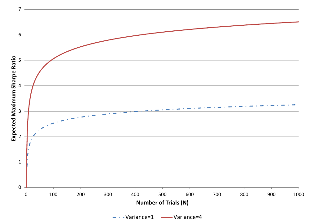
How to read it. Horizontally, the number of independent trials up to 1,000; vertically, the expected maximum Sharpe at a mean of 0. The blue dashed line is for a variance of Sharpe ratios of 1, the red one for a variance of 4.
What to notice. The curve rises quickly up to a hundred trials and slowly after that: by 1,000 trials it is about 3.3 at variance 1 and about 6.5 at variance 4.
The practical takeaway. The spread of Sharpe ratios between variants matters no less than their number: a standard deviation of Sharpe ratios twice as large (variance 4 instead of 1) raises the threshold twice as high.
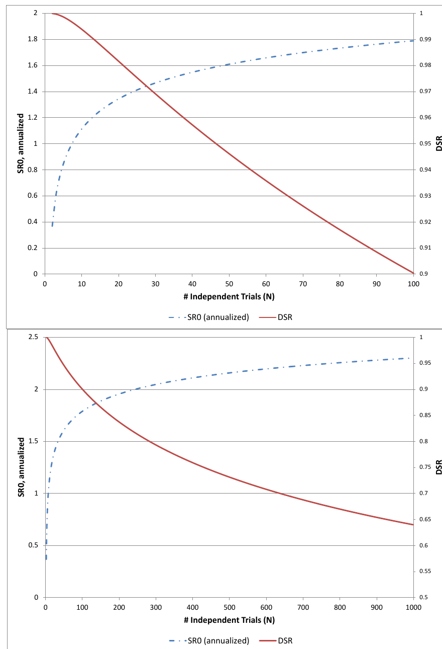
How to read it. Two panels for the same example: up to 100 and up to 1,000 trials. The blue dashed line is the threshold in annualized terms (left scale), the red line is DSR (right scale).
What to notice. On the upper panel DSR falls below 0.95 at around 46 trials and reaches 0.90 by a hundred. On the lower one, by a thousand trials DSR is about 0.64 (our calculation by the formula gives 0.640).
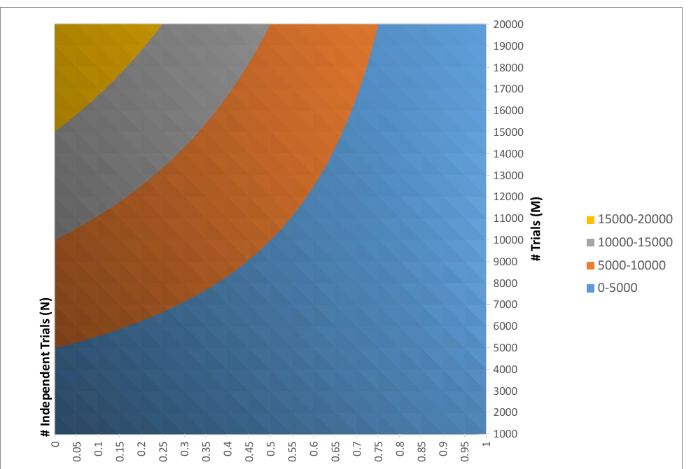
The number of independent trials. If the trials are correlated, is smaller than the number actually run (). Through the average correlation , the authors propose the interpolation
What this is. At correlation 0 all trials are independent, at correlation 1 there is effectively one trial; in between, the dependence is linear.
An example, our calculation. , : .
and they note its weaknesses themselves: correlation captures only linear dependence, and when the number of trials exceeds the length of the series, the correlation matrix is ill-conditioned and the estimate of the average correlation is itself overfit. As an alternative they mention methods from information theory.
When to stop. The authors propose an optimal stopping rule (“the secretary problem”, the law): out of the theoretically grounded configurations, randomly choose and test about 37 %, then test them one at a time and stop at the first one that is better than all the previous ones. This is a heuristic from a different problem; the authors themselves note in a footnote that in choosing a strategy, unlike in the original problem, one can go back to an earlier candidate.
4. The paper's check of the maximum formula
The authors compare the approximation with a simulation on a “mean × number of trials” grid, with 10,000 repetitions each (appendix A.2, Exhibits 3.1 and 3.2).
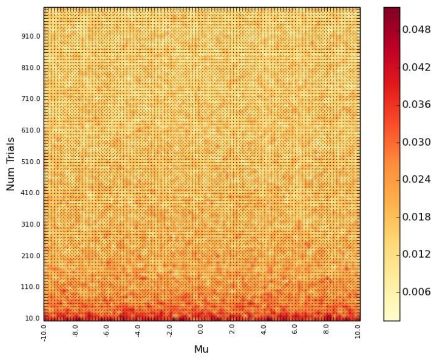
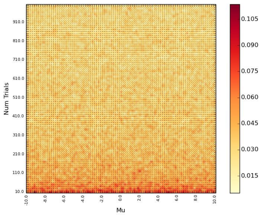
How to read them. Horizontally, the mean of the Sharpe ratios (Mu); vertically, the number of trials from 10 to 1,000; the color is the error “approximation minus simulation”. At the bottom, with a small number of trials, the error is up to 0.05 (variance 1) and up to 0.11 (variance 4); higher up the color is even, about 0.012–0.018.
What to notice. The error does not depend on the mean (the bands are horizontal) and is always positive: the approximation slightly overstates the maximum, so the threshold is a little stricter than needed.
5. What is shaky in the paper
What turned up in the cross-check
The numerical example reproduces to the fourth decimal place. , DSR 0.9004, at DSR 0.9505, with normal returns and also 0.9505; these are the largest at which DSR is not below 0.95.
The code and the figure disagree on the range. In Snippet 1 the mean is iterated as np.linspace(-100,100,101), that is, from −100 to 100, while on the heat maps of Exhibits 3.1 and 3.2 the Mu axis runs from −10 to 10. The figure was not built with the attached code, or the code was edited afterwards. This does not affect the conclusion: the error does not depend on the mean.
Only this goes into the paper's count of discrepancies (the field on the site): the paper disagreeing with itself. Everything below is our check, not a contradiction within the text.
Our check, which the paper does not have
The precision of the approximation is worse than stated. The authors: "by 1000 trials it is as small as 0.006 for a process with variance 1" and "The error quickly converges to zero as the number of trials grows". We computed the exact expectation of the maximum by numerical integration: the approximation error is +0.036 at 10 trials, +0.023 at 100, +0.014 at 1,000. It decreases slowly. The figure 0.006 is, in all likelihood, the minimum over the cells of the heat map, where each cell is noisy from the simulation (a standard error of about 0.004), while the typical color of the map at large is exactly 0.012–0.018. The error is on the safe side; the threshold is slightly overstated.
Formula (9) counts the correlation twice if the variance of Sharpe ratios is taken as the spread across trials. The paper defines as "the variance across the trials’ estimated SR", that is, the spread of Sharpe ratios between variants. With correlated trials, this spread is already smaller than the true variance of each Sharpe: the common part of the noise is the same for all of them and does not enter the spread. If, on top of that, the number of trials is also reduced by (9), the correlation is counted twice, the threshold is understated, and DSR comes out softer than it should.
Our experiment on a model with equal correlation between all trials, 1,000 trials without skill, 4,000 repetitions:
| Correlation | Actual mean maximum | with | The same with from (9) |
|---|---|---|---|
| 0.0 | 3.237 | 3.256 | 3.256 |
| 0.3 | 2.715 | 2.722 | 2.636 () |
| 0.5 | 2.280 | 2.301 | 2.158 () |
| 0.8 | 1.435 | 1.455 | 1.237 () |
All numbers are in units of the standard deviation of the Sharpe of a single trial. In this model, the right answer comes from with the spread across trials; adjustment (9) understates the threshold relative to it by 0.09, 0.14 and 0.22 at correlations of 0.3, 0.5 and 0.8. If, on the other hand, the variance is taken not as the spread across trials but as the theoretical variance of a single Sharpe, the effective should be much smaller than (9) gives. The linear interpolation (9) follows from neither; the authors do say that it is an interpolation between the extreme cases. Our conclusion; the equal-correlation model is ours.
Minor points
The caption of Exhibit 3.2 refers to "Exhibit 2.1", although 3.1 is meant. The title of appendix A.1: "EXPECTED MAXIMUM SHARE RATIO". In the text the American Statistical Association is called a “Society” and dated 1997, in the reference list 1999.
A subtlety in the wording. The authors write that the investor understood: "there is only a 90% chance that the true SR associated with this strategy is greater than zero". Formally, DSR is the probability of exceeding the threshold ; it can be read as “the chance that the true Sharpe is greater than zero” only within the paper's logic, where the threshold is zero adjusted for selection.
6. What follows in practice
Store the number of trials and the spread of their Sharpe ratios. Without these two numbers DSR cannot be computed. An optimizer that keeps only the winner makes the test impossible after the fact, just as for PBO.
Compute the Sharpe in units of one period and use full kurtosis. Plugging an annual Sharpe, or excess kurtosis instead of full kurtosis, into the formula means getting a meaningless result.
For a correlated parameter search, do not reduce by (9) if is the spread of Sharpe ratios between variants. On our model it is more honest to take equal to the number of runs.
Skewness is decisive. Strategies with rare large losses (selling volatility, averaging down) get a much smaller “trial budget” than trend strategies with positive skewness.
DSR and PBO complement each other. DSR is fast and needs five numbers, but it relies on the normality of Sharpe ratios across trials. PBO is nonparametric, but it needs the full return matrix of all variants.
7. Testable ideas
| No. | Idea | Type | Where to compute |
|---|---|---|---|
| 1 | Compute DSR for each finalist: the threshold from the number of independent trials and the spread of Sharpe ratios of all trials, cutoff 0.95 | acceptance metric | Python |
| 2 | A search log: the number of trials and the Sharpe of each, so that the spread can be computed later; without it DSR cannot be recovered | audit | any |
| 3 | Do not reduce by formula (9) if is taken as the spread of Sharpe ratios between trials: the correlation is counted twice and DSR comes out softer | audit | Python |
| 4 | Plug in the per-period Sharpe, not the annual one, and full kurtosis (3 for the normal); check on your own strategies how much skewness cuts the allowable number of trials (in the example from 88 to 46) | diagnostic | Python |
| 5 | A quick threshold for the “best-by-chance” trial: the expected maximum of standard normals (2.53 at 100, 3.26 at 1,000) multiplied by the spread of Sharpe ratios in the search | diagnostic | any |
| 6 | Test the stopping rule on your own searches: how many trials it saves and whether it loses a real effect | design change | Python |
| 7 | Compute both DSR and PBO on the same search and examine the cases where they disagree | acceptance metric | Python |