How to read this walk-through. The main idea of the paper fits into one picture: Figure 1 in section 3. The mechanism and the formulas are in section 2, the practical part (costs, leverage) in section 6, the weak spots in section 9. The theoretical section 8 can be skipped if only trading is of interest. We did not recompute the paper's numbers; examples on numbers the authors do not give are marked as ours.
The main thesis
The authors take ready-made factor portfolios (the stock market, value, momentum, profitability and others) and each month scale them in inverse proportion to the realized variance of the previous month. The previous month was turbulent, the position is smaller; calm, larger. This managed version gives a significant positive alpha against the original factor for most of the nine factors.
The explanation in one sentence: volatility is highly predictable at a short horizon, while expected return is barely related to it, so the ratio “return per unit of risk” is worse in turbulent months, and a sensible investor should cut back in those months.
The authors themselves stress the uncomfortable side of the result: the strategy reduces risk in recessions, crises and after crashes, that is, exactly when the conventional advice is to hold the position or add to it. In the autumn of 2008 the strategy went almost entirely to cash and came back when volatility subsided. In the authors' view this rules out the usual risk-based explanations and challenges structural models of time-varying expected returns.
1. How it works: the factor, the price of risk and timing
What a factor is in this paper. Not a fund and not a trading system, but a published return series of an academic strategy. Mkt: the whole stock market over the bill rate. SMB: small companies against large ones. HML: cheap by book value against expensive. Mom: winners of the past year against losers. RMW: profitable against unprofitable. CMA: conservatively investing against aggressive. ROE and IA: return on equity and investment from the Hou, Xue and Zhang model. Carry: high-rate currencies against low-rate currencies.
Data: daily and monthly factors from Ken French's website, the Hou–Xue–Zhang factors, and the Lustig–Roussanov–Verdelhan currency carry obtained from Adrien Verdelhan. The periods differ: 1926–2015 for Mkt, SMB, HML and Mom, 1963–2015 for RMW and CMA, 1967–2015 for ROE and IA, 1983–2015 for carry.
The authors' starting point: a mean-variance investor holds more of the risky asset the better the ratio of expected return to variance, . At a monthly horizon the numerator is predicted poorly, the denominator well. If the numerator is taken as roughly constant, what remains is to divide by the variance forecast.
It is important to distinguish this from how volatility is used in most systematic strategies. Usually dividing by volatility equalizes quiet and turbulent instruments with each other. Here one and the same portfolio is held at different sizes in different months: this is timing over time, not normalization across instruments. The paper justifies precisely the second.
2. The method in one line
Each month multiply the factor's return by divided by the variance of its daily returns over the previous month; then check by a regression on the original factor whether any alpha remains.
What this is. A position sizing rule: the more it shook last month, the less risk this month.
What each symbol means.
- : the return of the original factor (“just hold”) in the next month.
- : the return of the managed version. The superscript (“sigma”) is only a label, not a power.
- (“sigma hat squared”): the variance estimate from the previous month. The hat means an estimate.
- : a constant multiplier chosen so that the managed version has the same unconditional volatility as the original.
Step by step. At the end of the month compute the variance of the factor's daily returns over that month. Divide by it; this is the weight for the next month. Multiply the weight by the next month's return.
Our example. Suppose that after choosing the weight in a calm month came out at 2.0, and in a month with four times the variance at 0.5. In the calm month we are at double size, in the turbulent one at half size.
Why the constant is needed. To keep the comparison fair: otherwise an “improvement” could be obtained simply by increasing the average bet size. The authors note that fitting over the full sample does not look into the future in any sense that matters for the Sharpe ratio:
"c has no effect on our strategy’s Sharpe ratio"(footnote 5).
What this is. Realized variance: how scattered the factor's daily returns were within the previous month.
What each symbol means. : the number of the trading day in the month; the authors use 22 days. : the factor's return on that day. The inner sum divided by 22 is the average daily return over the month. The outer sum adds up the squared deviations from the average.
Step by step. Take the daily returns for the month, find their average, find each one's deviation from the average, square it, add them up.
Our example, on five days. Returns +1, −2, +0.5, −1, +1.5 %. The average is 0. Squared deviations . If the days had been +0.2, −0.3, +0.1, −0.2, +0.2 %, the sum would be 0.22, almost 40 times smaller, and the weight for the next month that many times larger.
Why this matters. No models and no estimated parameters. The authors stress that an investor could act this way in real time. More sophisticated variance forecasts in the appendix give a better result, but the main line rests on the simplest version.
What this is. A check of whether the managed version added anything beyond the original factor.
What each symbol means. (“beta”): how closely the managed version follows the original. (“alpha”): what the regression did not explain, the timing's own contribution. (“epsilon”): noise.
Why this matters. A positive alpha means that the combination “original factor plus managed version” has a higher Sharpe ratio than any static share of the original factor combined with cash. If the factor describes the prices of a wide range of assets well, this is an expansion of the whole efficient frontier.
What this is. The left formula: what Sharpe ratio the investor gets by adding the managed version to the original. The right one: by how many percent the utility of a mean-variance investor grows.
What each symbol means. : the Sharpe ratio of the original factor. : the standard deviation of the regression residuals (in the paper's tables this is RMSE). : the appraisal ratio, alpha per unit of added risk.
Step by step. Square the Sharpe ratio and the appraisal ratio, add them, take the square root. The squares add because the alpha and the original factor are uncorrelated by construction, like the legs of a right triangle.
A worked example on the paper's numbers, our calculation. For the market the original Sharpe ratio is 0.42, the appraisal ratio 0.33. ; in Table 5 of the paper the Sharpe ratio of the managed market is 0.52, an increase of about 25 %. The utility gain on these rounded numbers is about 60 %; the authors give 65 %.
A subtlety with annualizing. The authors multiply monthly returns by 12, and then volatility also grows 12 times, so the ratio stays monthly: the appraisal ratio is additionally multiplied by (footnote 9). Their example: for momentum the alpha is 12.5 and RMSE about 50, appraisal .
3. Results by individual factor
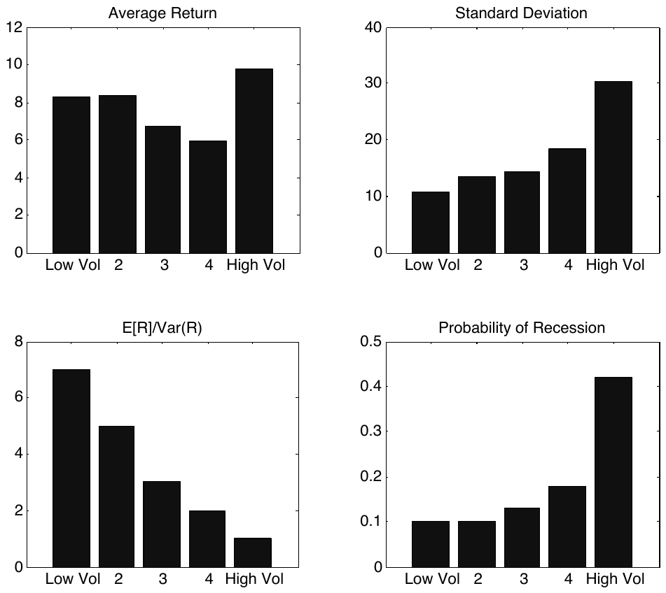
How to read it. All months are split into five groups by the market's realized volatility in the previous month, from Low Vol (the calm 20 %) to High Vol (the turbulent 20 %). For each group the chart shows what happened in the following month.
What to notice. The average return (top left) jumps around with no order: roughly 8.3, 8.4, 6.7, 5.9 and 9.8 % a year. Volatility (top right) rises like a staircase: roughly 10.8, 13.4, 14.2, 18.4 and 30.2 %. Their ratio (bottom left) therefore falls from 7.0 to 1.0. The probability of recession (bottom right) in the turbulent group is about 0.42 against 0.10 in the calm one.
The practical takeaway. Risk is predictable, the reward for it at a monthly horizon is not. In turbulent months the deal is worse, and cutting back is sensible, and the cutting back will happen precisely in recessions.
Table 1 of the paper, alphas of the managed factors against the originals (annual, in percent, standard errors in parentheses).
| Mkt | SMB | HML | Mom | RMW | CMA | Carry | ROE | IA | |
|---|---|---|---|---|---|---|---|---|---|
| Beta to the original | 0.61 | 0.62 | 0.57 | 0.47 | 0.62 | 0.68 | 0.71 | 0.63 | 0.68 |
| Alpha | 4.86 (1.56) | −0.58 (0.91) | 1.97 (1.02) | 12.51 (1.71) | 2.44 (0.83) | 0.38 (0.67) | 2.78 (1.49) | 5.48 (0.97) | 1.55 (0.67) |
| Alpha controlling for the three Fama–French factors | 5.45 | −0.33 | 2.66 | 10.52 | 3.18 | −0.01 | 2.54 | 5.76 | 1.14 |
| Observations, months | 1,065 | 1,065 | 1,065 | 1,060 | 621 | 621 | 360 | 575 | 575 |
| RMSE | 51.39 | 30.44 | 34.92 | 50.37 | 20.16 | 17.55 | 25.34 | 23.69 | 16.58 |
How to check significance in your head. Divide the alpha by the standard error in parentheses: more than two roughly means significance. Market , momentum , CMA , nothing. Our calculation.
Where the effect is strongest. Momentum: 12.51 % a year, appraisal ratio 0.875. The authors link this to the work of Barroso and Santa-Clara: strategies that avoid momentum crashes by timing its volatility work exceptionally well. Appraisal ratios in the paper's text: market 0.34 (0.33 in the introduction and Table 2), HML 0.20, profitability 0.41, carry 0.44, ROE 0.80, investment 0.32.
Where there is no effect. SMB: the alpha is negative and insignificant. CMA: about zero.
A separate caveat from the authors on tradability: an ordinary investor could replicate the managed market in real time, but momentum is harder: "The typical investor will likely find it difficult to trade the momentum factor" (footnote 7).
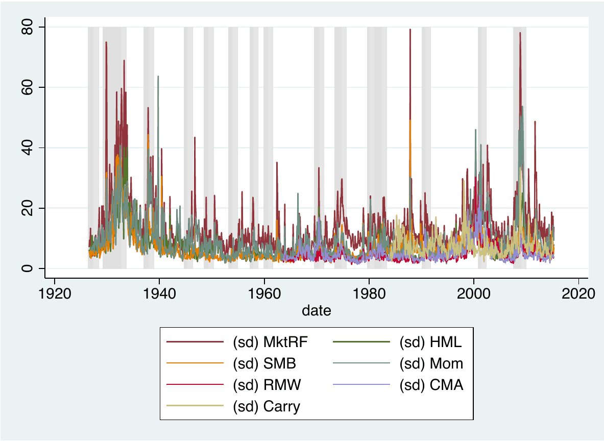
How to read it. Lines of different colors: the monthly volatility of each factor in percent a year. Gray bars are recessions as dated by the NBER.
What to notice. Volatility comes in patches: calm periods last for years, and so do turbulent ones. The spikes fall in the 1930s, 1987, 2000–2002 and 2008, and for all factors at once. It is this clustering that makes the previous month a usable forecast of the next one, and the dynamics shared across factors explain the result of section 7 on common volatility.
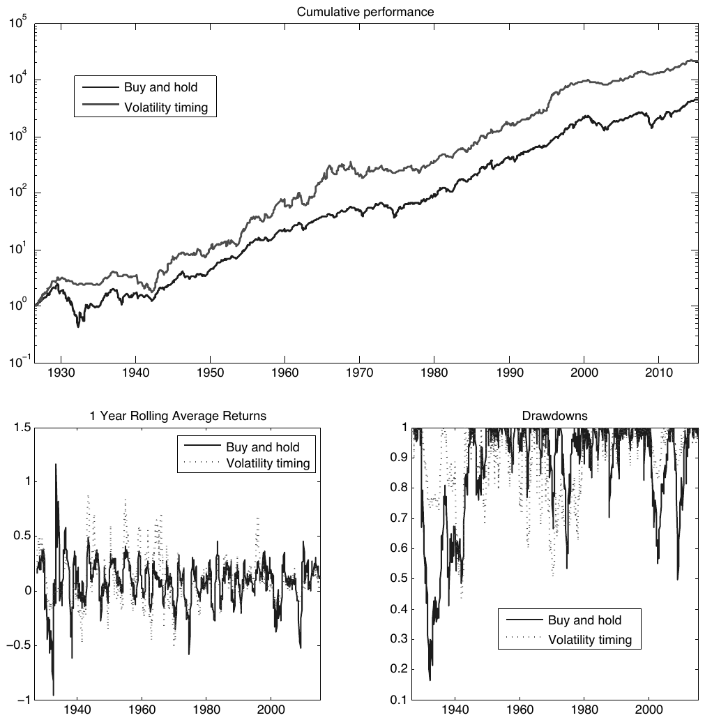
How to read it. At the top, the cumulative result of one dollar invested in 1926, on a log scale; both versions have the same unconditional volatility. Bottom left, rolling annual returns; bottom right, drawdowns.
What to notice. According to the paper's text, by the end of the sample the managed version gave about $20,000 against roughly $4,000. It loses in calm low-volatility periods (for example, the 1960s), when it runs with increased leverage, and avoids the big crashes (the Great Depression, 2008), because by their peak it has already cut back.
What else is visible. On the drawdown panel the managed version has deep drawdowns of its own, about half of capital in the early 1940s and around 1970. The worst periods of the strategy and of the market do not coincide, but it does have its own slumps.
4. Factor combinations and subsamples
A stricter test: what if the investor already has all the factors and has built the best static combination of them (MVE, mean-variance efficient)? The authors time this combination as a whole, without changing the relative weights of the factors.
Table 2 of the paper, panel A.
| Mkt | FF3 | FF3 + Mom | FF5 | FF5 + Mom | HXZ | HXZ + Mom | |
|---|---|---|---|---|---|---|---|
| Alpha | 4.86 | 4.99 | 4.04 | 1.34 | 2.01 | 2.32 | 2.51 |
| Standard error of alpha | 1.56 | 1.00 | 0.57 | 0.32 | 0.39 | 0.38 | 0.44 |
| Sharpe of the original combination | 0.42 | 0.69 | 1.09 | 1.20 | 1.42 | 1.69 | 1.73 |
| Appraisal ratio | 0.33 | 0.50 | 0.69 | 0.56 | 0.77 | 0.91 | 0.91 |
The combination weights are fitted over the full sample. The authors note that because of this "the original MVE Sharpe ratios are likely to be overstated relative to the truth" (section 2.5), and so, in their words, the Sharpe gain is if anything understated.
Table 2 of the paper, panel B, alpha by thirty-year periods.
| Mkt | FF3 | FF3 + Mom | FF5 | FF5 + Mom | HXZ | HXZ + Mom | |
|---|---|---|---|---|---|---|---|
| 1926–1955 | 8.11 (3.09) | 1.94 (0.92) | 2.45 (0.74) | ||||
| 1956–1985 | 2.06 (2.82) | 0.99 (1.43) | 2.54 (1.16) | 0.13 (0.43) | 0.71 (0.67) | 0.77 (0.39) | 1.00 (0.51) |
| 1986–2015 | 4.22 (1.66) | 5.66 (1.74) | 4.98 (0.95) | 1.88 (0.41) | 2.65 (0.47) | 3.03 (0.50) | 3.24 (0.57) |
The middle period is weaker: for the market the alpha is 2.06 with a standard error of 2.82, that is, insignificant. The point estimates are positive everywhere. The authors' explanation: timing works only when volatility fluctuates strongly, and "Volatility varied far less in the 1956-1986 period" (section 2.5; so in the text, although the period in the table is 1956–1985).
5. Recessions, dynamics and horizon
What this is. The same regression, but with a switch for recession months.
What each symbol means. : an indicator equal to 1 in NBER recession months and 0 otherwise. : the beta in normal months. : how much the beta in a recession differs from the normal one; in a recession the beta equals .
A worked example on the paper's numbers. For the market , , so in a recession it is .
Why this matters. To test the explanation “the strategy makes money because it takes recession risk”. The opposite comes out: in recessions the risk is lower.
According to Table 3 of the paper, is negative for all factors tested in the table (SMB is not in it): HML −0.43, Mom −0.53, CMA −0.41, ROE −0.42, IA −0.39. For RMW (−0.08 with a standard error of 0.13) and for carry (−0.26 with a standard error of 0.15) the difference is weak.
How to reconcile this with expected returns being high in recessions. The authors build a vector autoregression (VAR) from realized variance, returns and Shiller's CAPE and look at how the system responds to a variance shock.
What a VAR is, in plain terms. A model in which several quantities explain each other with a lag. The system is given a single push, and one watches how each quantity reacts and how long it takes to return to normal. This is called the impulse response.
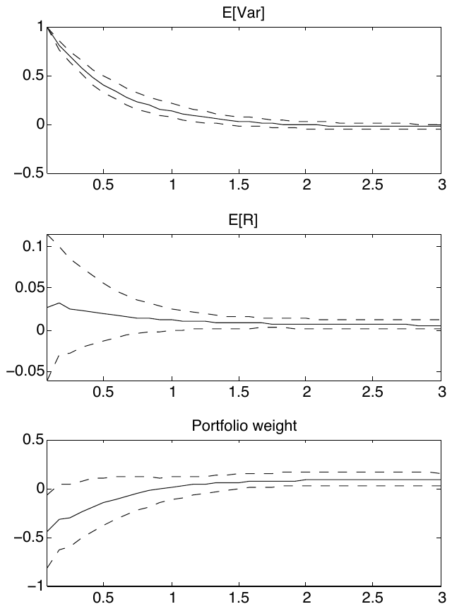
How to read it. Three panels, years after the shock on the horizontal axis. At the top, expected variance; in the middle, expected return; at the bottom, the optimal weight of a mean-variance investor in deviations from the average. The dashed lines are confidence intervals.
What to notice. Variance jumps and returns almost to normal in a little over a year. Expected return rises weakly but stays up longer. The weight is cut roughly in half right after the shock and comes back after roughly a year: according to the paper's text, the share stays below one for about 12 months.
What else is visible. The lower bound of the interval for expected return is below zero in the first months: the rise in returns after the shock is not statistically established. The authors themselves warn that the return response
"should be read with caution, as return predictability regressions are poorly estimated"(section 3.6).
The authors' conclusion: both facts are true, but at different speeds. Volatility jumps sharply and goes away quickly, while expected return rises more weakly and stays up for a long time. So right after the shock it is sensible to cut back and then gradually return, and that is what the strategy does.
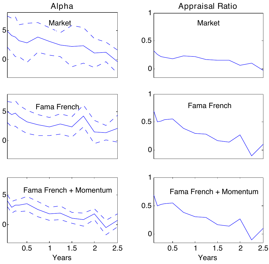
How to read it. The weight is computed from the variance of the last month, but the position is held for months without recalculation. Horizon in years on the horizontal axis; on the left, alpha with a 90-percent interval, on the right, the appraisal ratio.
What to notice. Both quantities slowly decline as the horizon lengthens: past volatility predicts a distant period worse. According to the paper's text, the market alpha is significant at the 10-percent level up to 18 months.
What else is visible. On the top left panel the lower bound of the interval for the market touches zero already at about half a year, so “up to 18 months” should be read as “significant at most points up to 18 months”. The authors add that the VAR gives an almost zero autocorrelation of volatility at 12 months, while the nonparametric estimate is above 0.2, so the alpha falls more slowly than the VAR suggests.
6. Costs and leverage
Table 4 of the paper, the market portfolio. is the average absolute change in the weight over a month. 1 bp is taken from Fleming and coauthors, 10 bp from Frazzini and coauthors for trading about 1 % of daily volume, 14 bp adds 4 bp for the rise in costs when the VIX is at the 98th percentile. The last column: at what costs the alpha goes to zero.
| Weight | Description | E[R], % | α, % | α at 1 bp | α at 10 bp | α at 14 bp | Break-even, bp | |
|---|---|---|---|---|---|---|---|---|
| realized variance | 0.73 | 9.47 | 4.86 | 4.77 | 3.98 | 3.63 | 56 | |
| realized volatility | 0.38 | 9.84 | 3.85 | 3.80 | 3.39 | 3.21 | 84 | |
| AR(1) variance forecast | 0.37 | 9.47 | 3.30 | 3.26 | 2.86 | 2.68 | 74 | |
| no leverage | 0.16 | 5.61 | 2.12 | 2.10 | 1.93 | 1.85 | 110 | |
| leverage up to 50 % | 0.16 | 7.18 | 3.10 | 3.08 | 2.91 | 2.83 | 161 |
What matters here. Dividing by volatility instead of variance halves turnover (0.38 against 0.73) and raises the break-even threshold from 56 to 84 bp. The reason is arithmetic: variance is the square of volatility, and dividing by it reacts to changes twice as sharply. Capping leverage cuts turnover 4.5 times, the alpha falls to 2.12–3.10 %, and the break-even threshold rises to 110–161 bp.
What break-even costs are. A single number that tells whether there is a safety margin, without arguing about which cost model is right. In the authors' words, the strategy
"survives transactions costs, even in high volatility episodes"(section 3.2).What is missing here. Costs are computed only for the market: for the other factors, according to the authors, there are no good estimates even of the cost of trading the factor itself.
Leverage (Table 5 of the paper). The distribution of the base strategy's weight: median 0.93, 75th percentile 1.59, 90th 2.64, 99th 6.39. For the version that divides by volatility the 99th percentile is 3.36, for the AR(1) forecast 4.58. The Sharpe ratio of all variants, including the capped ones, is almost the same: 0.51–0.53.
Why the upper percentiles matter more than the median. A median of 0.93 looks harmless. But in one month out of a hundred the base strategy needs more than sixfold leverage, and in the calmest months at that. If the broker will not provide that much, the strategy does not work the way it does in the table.
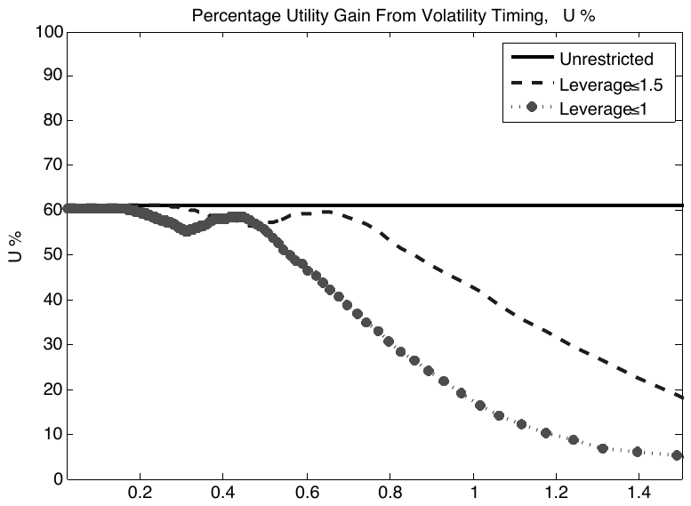
How to read it. On the horizontal axis, the investor's target unconditional equity share (the lower the fear of risk, the higher it is); on the vertical axis, the utility gain in percent. The solid line is unconstrained, the dashed line is leverage up to 1.5, the dots are no leverage.
What to notice. Without constraints the gain is about 60 % at any target share. With constraints the gain depends strongly on how much risk the investor wants: at a target share of 0.6 and a ban on leverage about 50 %, at a share of 1.0 and leverage up to 1.5 about 45 % (both numbers in the paper's text), and at a share of 1.0 with a ban on leverage only about 17 % on the chart. For an investor who wants to be fully in equities anyway, the ban on leverage eats most of the gain.
Leverage through options. To answer the objection “it is all about access to leverage”, the authors implement the increased exposure through a portfolio of six in-the-money calls on the S&P 500 (60 and 90 days, beta about 7), April 1986 to January 2012. Sharpe ratio: “just hold” 0.39, ordinary timing 0.59, through calls 0.54, through calls and sold puts 0.60. Alphas 4.03, 5.90 and 6.67 with standard errors 1.81, 3.01 and 2.86.
Utility. An investor with access only to the market raises utility by 65 % by the authors' calculation; according to the estimate of Campbell and Thompson, timing expected returns gives about 35 %. From Figure 4, without constraints, about 60 %; the authors explain the difference by a different setup (footnote 11).
7. Robustness checks
Risk parity and betting against beta. These are cross-sectional strategies: at a given moment they prefer calm assets to turbulent ones. Here the timing is over time: one and the same portfolio at different times. Controlling for the risk parity factor does not change the alpha (4.86 → 4.86 for the market), nor does controlling for BAB (appendix, Table 9), and the volatility-managed version of BAB itself gives an alpha of 5.67 % against the original BAB.
Common volatility instead of its own (Table 7). If each factor is divided not by its own variance but by the first principal component of the variances of all factors, the results are slightly weaker but mostly the same: market 4.22, momentum 11.00, ROE 4.21. The exception is carry: "the alpha for the currency carry trade disappears" (section 3.5), alpha −1.28. The volatility of currency carry lives separately from equities.
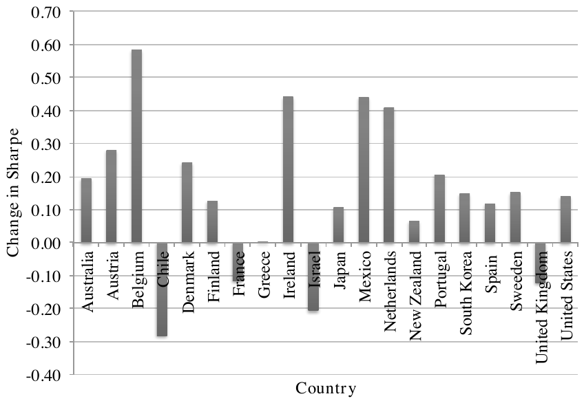
How to read it. A bar: the Sharpe ratio of a country's managed index minus the Sharpe ratio of “just hold”. Indices from Global Financial Data, in dollars, over the US rate.
What to notice. On average the Sharpe ratio is higher by 0.15, with a positive change in 80 % of countries. Negative for Chile, France, Israel and the United Kingdom, about zero for Greece, largest for Belgium (about 0.58).
The authors' caveat. Many series are prices only, without dividends, so
"our results are not intended to accurately capture the level of Sharpe ratios"(caption of Figure 8); in their view this affects the difference in Sharpe ratios only weakly.
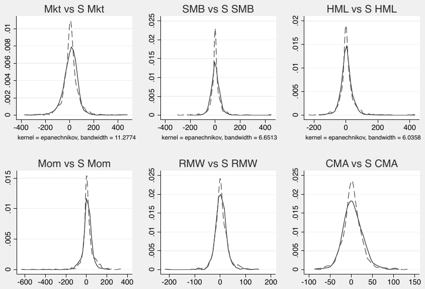
How to read it. The solid line is the distribution of the original factor, the dashed line that of the managed one.
What this tests. The objection “you sold crash insurance”: many strategies raise the Sharpe ratio at the expense of rare disasters, and then the left tail of the managed version would be fatter. On the chart the dashed line is more peaked in the center, and the tails are not fatter; the authors write that there is no clear pattern, and if anything is visible, then for some factors the left tail of the managed version is even thinner.
Other material from the appendix. The downside beta of the managed market is 0.11 and insignificant. The strategy is less sensitive to volatility shocks than the original factor, because in turbulent periods it holds less. By the manipulation-proof performance measure (MPPM, Goetzmann and coauthors) the managed market gives 4.33 % against 2.48 % for the market. On artificial data where the price of risk is constant, the MPPM of the managed version exceeds the market's in only 0.2 % of simulations, the median alpha is about 10 bp, and the chance of getting 4.86 % is practically zero.
Controlling for all factors at once (appendix, Tables 10 and 11). Here is an important caveat from the authors themselves: "Notably, the alpha for the scaled market portfolio is reduced when including all other factors" (Appendix A.3). Controlling for the market, HML, SMB and momentum (1926–2015), the alpha of the managed market is 2.43 with a standard error of 1.60; controlling for six factors (1963–2015), 0.18 with a standard error of 1.87. The authors explain this by part of the information in the managed market being contained in momentum, and consider the MVE combination from Table 2 the right benchmark for an investor with all the factors.
8. Theory: alpha as the covariance of the price of risk and variance
What this is. A formula that turns a trading result into a statement about how the market works: the alpha of timing equals, with a minus sign, the covariance of the “price of risk” and variance.
What each symbol means.
- (“mu”): the expected excess return at time .
- : the conditional variance.
- : the price of risk, the return per unit of variance. In Figure 1 this is the third panel.
- : covariance, whether two quantities move together. Positive: they rise together. Negative: one rises, the other falls.
- : the average over time.
How it reads in words. The alpha is positive when the price of risk is lower in periods of high variance. If the market paid proportionally more for risk in turbulent times (), the price of risk would be constant, the covariance zero, and there would be no alpha: by leaving turbulent periods the strategy would lose exactly as much return as risk.
A special case. If expected return is constant, the alpha equals , where . This is a Jensen's inequality term, and it grows with the volatility of volatility: the more variance wanders, the larger the alpha of timing.
Our example. Variance is 1 half of the time and 4 the other half (in arbitrary units). Then , , . If variance did not change, .
Why this matters. Standard models work the other way round: in bad times effective risk aversion rises, and the price of risk rises together with volatility. Then the covariance is positive, and the alpha is zero or negative.
Next the authors show how to recover from the alpha the part of the variation in the price of risk that is linked to volatility, and how to build a stochastic discount factor that prices both static and volatility-managed strategies. On the market's numbers, with the estimate of return predictability from Campbell and Thompson, accounting for changes in volatility reduces the squared pricing error by about 38 %, and accounting for changes in expected return by 21 %.
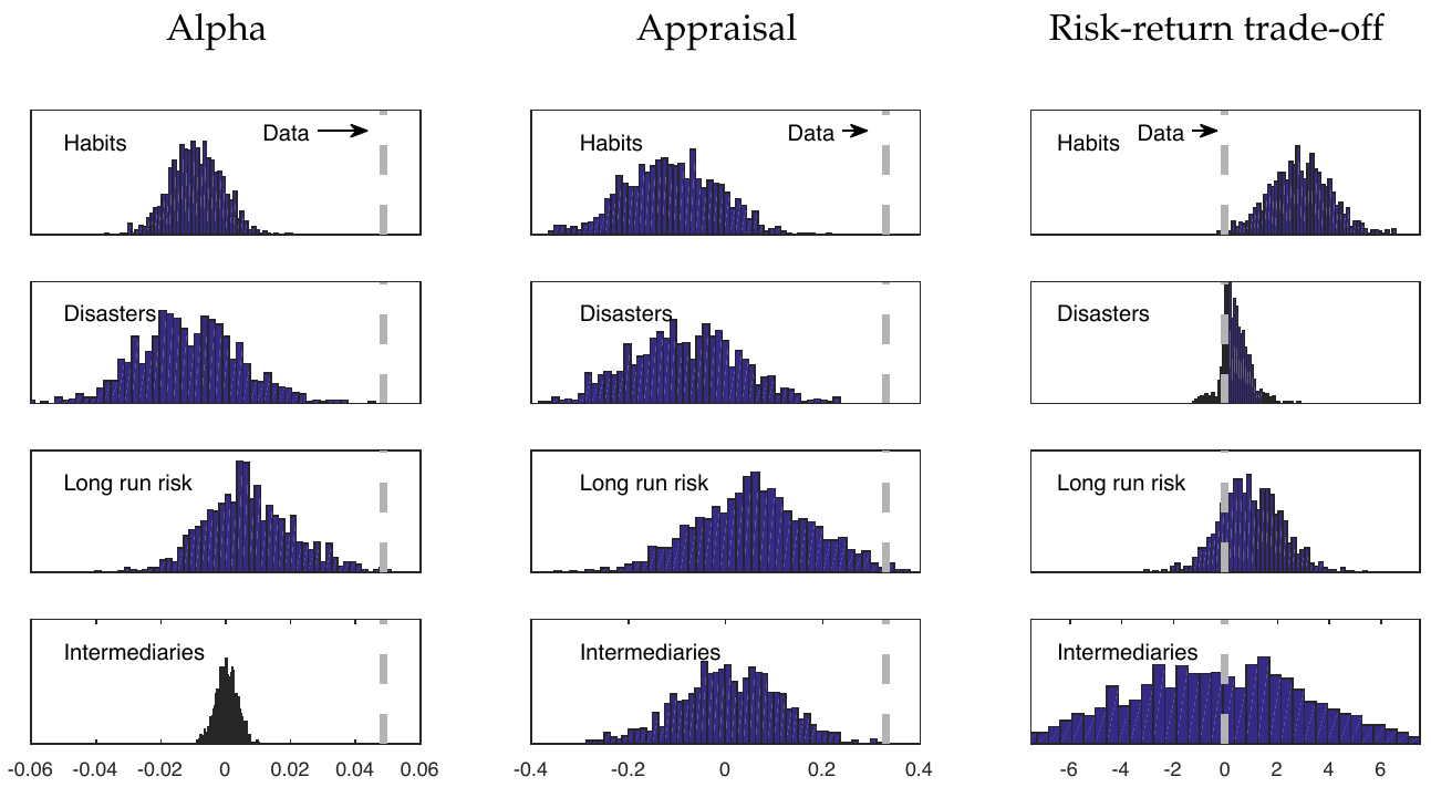
How to read it. Rows are the models: habit (Campbell–Cochrane), rare disasters (Wachter), long-run risk (Bansal–Yaron), intermediaries (He–Krishnamurthy). Columns: the alpha of the managed strategy, the appraisal ratio, and the coefficient of the ordinary regression “return on past variance”. The histogram shows what the model generates over 1000 artificial histories of 100 years each; the gray dashed line shows what is in the real data.
What to notice. For the alpha and the appraisal ratio the real value lies at the right edge or beyond all four distributions. For the ordinary regression (the right column) the real value near zero is easily compatible with the models. Hence the authors' thesis: their test is stricter than the ordinary regression of returns on volatility. According to the paper's text, the Bansal–Yaron model gives an equally large alpha
"only in 0.2% of the simulated samples"(section 5.1), the others even more rarely.
The authors explicitly leave open what could explain the result: "A definitive answer to this question is beyond the scope of this paper" (section 5.2). They list possibilities: investors trade slowly or update their view of volatility slowly; in turbulent periods the composition of shocks changes (more discount rate shocks, which a long-term investor can wait out); volatility from learning about structural parameters is priced differently from ordinary risk.
9. What is shaky in the paper
Caveats the authors make themselves
Unevenness across periods. In 1956–1985 the market alpha is 2.06 with a standard error of 2.82; the authors explain this by weak volatility fluctuations in that period.
Controlling for all factors. In the appendix the alpha of the managed market, when controlling for the other factors, above all momentum, falls to 2.43 (1926–2015) and 0.18 (1963–2015). The strong conclusion for the market applies to an investor who has only the market.
Combination weights over the full sample. The Sharpe ratios of the original MVE combinations, in the authors' words, are overstated because the weights are fitted in-sample. They conclude that the gain from timing is, if anything, understated because of this.
Tradability. Momentum and other long-short factors are hard for an ordinary investor to replicate, and costs are estimated only for the market.
The return response in the VAR. The authors themselves ask to read it with caution: return predictability regressions are poorly estimated.
The explanation of the effect. The authors give no definitive answer as to why the price of risk falls when volatility rises, and leave it for future work.
What is known outside the paper
The paper gave rise to a separate line of criticism. The best known is the article by Cederburg, O'Doherty, Wang and Yan “On the Performance of Volatility-Managed Portfolios” (Journal of Financial Economics, 2020): by their conclusion, in a strictly out-of-sample implementation, when the weights of the combination of the managed and original factor are estimated only from past data, the advantage disappears or becomes insignificant for most factors. This does not cancel the relationship observed in the data in Figure 1, but it means that the numbers in the tables cannot be carried directly into expectations. A neighboring paper by Harvey and coauthors (2018) shows that the Sharpe gain from volatility targeting exists for equities and credit, but not for bonds, currencies and commodities.
What we noticed on reading, without recomputing
These are discrepancies within the paper itself, found by comparing its tables and captions. We did not compute them, they do not affect the main conclusion, and so they are not included in the discrepancy count.
The alphas of two variants in Tables 4 and 5 are swapped. In Table 4 the variant dividing by realized volatility has an alpha of 3.85, the AR(1) forecast 3.30. In Table 5 it is the other way round: realized volatility 3.30 (standard error 1.02), the forecast 3.85 (standard error 1.36). Which pair is correct cannot be established from the text. This matters for the practical comparison “volatility or variance”: the twofold difference in turnover does not depend on it, but the difference in alpha does.
The number of lags in the VAR. In the text of section 3.6 the VAR is estimated "with one lag of (log) realized variance", in the caption of Figure 5 "2 lags of each variable".
Figure 6. The right panels for the combination of the three Fama–French factors and for the same with momentum coincide point for point by eye, and the initial value of about 0.7 is closer to the appraisal ratio of the combination with momentum (0.69) from Table 2 than without it (0.50).
10. What follows in practice
The two roles of volatility should not be mixed. Dividing by volatility to make instruments comparable and dividing to time the overall exposure are one line in the code, but they rest on different evidence. By splitting them into two multipliers, each can be tested separately.
Inverse volatility is more practical than inverse variance. Turnover is half as high, the break-even threshold on costs is higher (84 against 56 bp), the tail of the required leverage is milder (99th percentile 3.4 against 6.4).
Look at the upper percentiles of the required leverage, not at the median. The strategy requires the most leverage in the quietest months. A leverage cap barely changes the Sharpe ratio, but it lowers the alpha and depends strongly on how much risk the account owner wants on average.
Break-even costs as a metric. A single number in basis points immediately tells whether there is a margin, and it is comparable across strategies.
Expect underperformance in a quiet rising market. The strategy loses to “just hold” in calm years, when it runs with increased leverage, and avoids crashes that are preceded by rising volatility. Monitoring of a live account is worth building with this in mind.
Test the premise on your own data, not the result of the tables. Sorting months by past volatility (Figure 1) shows whether a given market has what the effect rests on. If returns rise together with past volatility, timing will not help.
If the portfolio already has momentum, expect less. The alpha of the managed market in the paper's appendix falls noticeably when controlling for momentum.
11. Testable ideas
| No. | Idea | Type | Where to compute |
|---|---|---|---|
| 1 | Scale the overall exposure of your basket in inverse proportion to the realized variance (or volatility) of its own return over the previous month; report the alpha and the appraisal ratio from a regression on the original basket | design change | backtester |
| 2 | Compare three weights: , and a variance forecast; measure the average , the alpha and the costs at which the alpha goes to zero | diagnostic | Python |
| 3 | For every strategy with volatility targeting report the 50th, 75th, 90th and 99th percentiles of the required weight; introduce a cap and measure how much alpha it costs | acceptance metric | Python |
| 4 | Add break-even costs in basis points to all backtests: the level of costs at which the alpha or the profit goes to zero | acceptance metric | any |
| 5 | Repeat Figure 1 on your markets: split months into five groups by the previous month's volatility and compare the average return, volatility and their ratio in the following month | diagnostic | Python |
| 6 | Regression of the managed version on the original with an indicator of crisis months (recessions or months of extreme volatility): check that exposure in crises is really lower | diagnostic | Python |
| 7 | Run the timing with the weight recalculated weekly, monthly and quarterly and find the point where the gain stops covering costs | diagnostic | backtester |
| 8 | Compute the scaling constant and the weights of the combination of the managed and original versions from past data only (expanding window); if the alpha disappears, this is exactly the out-of-sample implementation problem | audit | Python |
| 9 | Add the momentum factor or your own trend basket to the regression of the managed version; compare the alpha with and without the control (in the paper, for the market, 4.86 against 2.43 and 0.18) | audit | Python |
| 10 | Compare dividing each market by its own volatility with dividing by the common volatility of the basket; markets whose alpha disappears under common volatility, like currency carry, should be run separately | diagnostic | Python |
| 11 | Separate in the code cross-instrument normalization and timing over time into two separate multipliers with separate parameters, so that they can be switched on one at a time | audit | any |