How to read this walk-through. The whole idea of the paper is explained by one numerical example from the authors, without formulas; it is in section 3. Section 2 gives it in one line. Sections 6 and 7 show how the hypothesis was tested and where it did not fit. Ready-made formulas for estimating the number of bets and the costs from dollar volume and volatility are collected in section 8. Limitations are in section 9.
1. How it works: bets and business time
Markets differ by orders of magnitude. One stock trades a million dollars a day, another two hundred million. Typical trade size, spread and execution costs differ as well. The paper proposes a hypothesis under which these differences almost vanish: stop measuring time in minutes and start measuring it by the arrival of new decisions about positions.
What a bet is. A portfolio manager's decision to take a long-term position of a certain size. It is not an order and not a trade:
"Bets are neither orders nor trades nor prints"(section 1). A manager has decided to buy 100,000 shares of IBM. The manager may buy 20,000 a day for five days in a row, and an algorithm will cut each daily order into hundreds of prints. There is one bet. If an analyst recommended a purchase to ten clients and each bought 10,000 shares, this too, in the authors' view, is one bet of 100,000: all ten purchases grew out of the same information and are not independent. That is why bets are almost impossible to reconstruct from the tape.What business time is. A clock that ticks with the arrival of each new bet. The authors call the rate at which bets arrive market velocity. In an active market the clock runs fast, in a quiet one slowly.
To link the unobservable bets to observable volume and volatility, the authors introduce two multipliers. The volume multiplier (“zeta”): how many units of trading volume one unit of bet volume generates. If all trades are bets, ; if everything passes through a single specialist, ; if positions wander between intermediaries, . The volatility multiplier (“psi”): what share of volatility is caused by bets rather than by news without trading. With and bets produce 64 % of return variance, and news the remaining 36 %. For the tests the authors assume that both multipliers are the same for all stocks and periods. This is an assumption, and the authors write plainly that if the multipliers correlate with volume and volatility, the estimates are biased.
The authors measure bet size not in shares and not in dollars but in the risk it transfers per unit of business time:
What this is. Bet size in dollars of risk per tick of business time.
What each symbol means. : the asset index, : the period; these are indices, not powers. : price. (“Q tilde”): bet size in shares; the tilde means “random variable”. (“sigma bar”): daily volatility caused by bets. (“gamma”): the expected number of bets per day. : volatility per tick of business time.
Step by step. Multiply the dollar size of the bet by the volatility over the time between two bets.
The authors' example (section 1). A bet of $400,000, daily volatility 2 %, 100 bets a day. Volatility per tick is , and dollars.
Why this matters. This way bet size does not depend on a split (twice as many shares at half the price, the same risk) or on leverage (stock volatility twice as high, price half as high). A bet of 10 million in one stock and a bet of 1 million in another can be compared.
2. The method in one line
Two hypotheses. Bet invariance: the distribution of is the same for all assets and periods. Transaction cost invariance: the dollar cost of executing a bet is the same function of .
The observable quantity through which everything is expressed is trading activity:
What this is. The total dollar risk that all participants transfer in one calendar day.
What each symbol means. : daily return volatility. : price. : volume in shares per day. : daily dollar volume.
The authors' example. The paper's benchmark stock: price $40, a million shares a day, volatility 2 %. dollars of risk per day. If dollar volume is 8 times larger at the same volatility, is also 8 times larger.
Why a product rather than dollar volume. Two markets with the same dollar volume and different volatility transfer different amounts of risk. Treasury bills with huge volume and almost zero volatility carry little risk, and this is exactly the example the authors give.
Bet invariance implies how the number and size of bets depend on activity:
What this is. The number of bets per day and the average bet size, expressed through activity.
What each symbol means. : bet activity, the same product but for the volume and volatility generated by bets; it is converted from the observed via the multipliers and . (“iota”): a constant common to all assets, . : the average bet size regardless of sign.
How it reads in words. Activity rose by 1 %, the number of bets rose by 2/3 %, their size by 1/3 %.
"As bet activity increases, the number of bets increases twice as fast as their size. This specific relationship between the number and size of bets lies at the very heart of invariance."(section 1).The authors' example. There are four times as many bets at the same daily volatility. Volatility per tick has halved, and for the risk per tick to stay the same, the bet must double. Dollar volume has grown times; , .
For traders, order size as a fraction of daily volume is more convenient. In these units the prediction is:
What this is. The distribution of bet size as a fraction of bet volume.
What means. “Equal in distribution”: what coincides is not a single value but the whole shape of the distribution.
Step by step. Take order size as a fraction of daily volume and multiply by activity to the power 2/3. The result is a quantity with the same distribution in any stock.
Why this matters. An order of 10 % of daily volume in a quiet stock and in an active one are different events. When activity grows 150 times, as between the extreme groups in the paper's data, the typical order's share of daily volume should fall by a factor of .
3. The authors' numerical example: the whole paper without formulas
The example from section 1 of the paper, close to the text.
Starting point. A stock with dollar volume of $40 million a day and daily volatility of 2 %. About 100 bets a day, the average bet $400,000.
Daily risk of the average bet. 2 % of 400,000, that is, $8,000: the standard deviation of the profit or loss of the average position over a calendar day.
A tick of business time. 100 bets a day means roughly one bet every 4 minutes. The clock ticks once every 4 minutes.
Risk per tick. Volatility over 4 minutes equals basis points. The risk of the average bet per tick is $800. The main claim: "Invariance implies that the specific number $800 is constant across stocks and across time."
The market becomes more active. Four times as many bets, 400 a day, with the same volatility. The clock ticks once a minute, and volatility per tick is bp. For the risk per tick to stay at $800, the average bet must grow to 800,000. Daily dollar volume grows from 40 to 320 million, 8 times.
Costs. Suppose executing the average bet costs $2,000, and this too is an invariant. In the first stock this is 50 bp of a $400,000 bet, in the second 25 bp of a $800,000 bet. At the same volatility, percentage costs fall in inverse proportion to dollar volume to the power 1/3.
The tail of the distribution. The same calculation for a 99th-percentile bet: risk per tick $10,000, size 5 million in the first stock and 10 million in the second; with costs of $50,000 this is 100 and 50 bp. The percentage spread will also halve.
Why the square root of the number of ticks. Volatility grows as the square root of time: over a period four times longer the dispersion is twice as large. Conversely, over 1/100 of a day volatility is 10 times smaller than daily volatility.
4. Costs: the illiquidity measure and the decomposition
The second hypothesis speaks of dollars, while traders count in basis points. The conversion gives a decomposition of percentage costs into two factors (the theorem in section 1):
What this is. The percentage cost of executing a bet of shares.
What each symbol means. : the illiquidity of a specific asset, the volume-weighted average execution cost in percent. : the cost shape function, the same for all assets. : bet size converted into risk per tick of business time.
The authors' example for . A manager executed 10 million at 20 bp, 5 million at 10 bp and 100 million at 80 bp. The volume-weighted cost is bp.
The authors' example for . A bet of average size costs 1.2 times the average cost: . A bet 5 times larger than average costs 10 times more: .
Why this matters. The cost curve differs strongly between stocks. If size is converted into and costs are divided by , all the curves should fall onto one.
Illiquidity is expressed through observable quantities:
What this is. The cube root of the ratio of return variance to dollar volume.
How to read it. The higher the volatility, the more expensive it is to trade; the larger the dollar volume, the cheaper. The symbol means “proportional to”: the multiplier is common to all assets.
Why the cube root. The authors explain it through leverage rather than a split:
"The cube root is necessary to make the illiquidity measure behave properly when leverage changes."If a stock is made twice as leveraged, the price halves, variance quadruples, and the ratio of variance to dollar volume grows 8 times. The risk transferred has not changed, so dollar costs have not changed either, while percentage costs must double, because the dollar size of the bet is half as large. The cube root turns 8 into 2.An example. Between the extreme volume groups in the paper's data, activity differs 150 times at almost the same volatility. The forecast is a fall in the spread and in percentage costs by a factor of .
The same reasoning yields a prediction for the quoted spread: , that is, at the same volatility an 8-fold rise in activity halves the percentage spread.
Invariance does not fix the shape of the function : "Invariance does not restrict the shape of this function; it can be consistent with either linear or square-root models of price impact." The authors test two shapes. Linear impact follows from adverse-selection models such as Kyle (1985). Square-root impact is consistent with econophysics, although, as the authors caution, "these results are based on single trades rather than bets". The square-root model has a special feature: impact in units of volatility depends only on the bet's share of volume, and, according to the authors, the square root is the only function with this property.
What the paper says about the Amihud measure
Section 2 shows how invariance closes a gap in the Kyle (1985) model: market depth there equals the ratio of price volatility to the volatility of order imbalance, and the imbalance is not visible in the data. If one assumes that all assets have the same number of bets, the result is a measure similar to Amihud's illiquidity, . The authors consider this assumption unrealistic: active stocks have more bets. There is also a technical problem: the Amihud measure has time units, and its value depends on the intervals over which volume and volatility are computed. The measure does not depend on time units. For the Amihud measure to give the same coefficient for all stocks, each stock would have to be computed over its own time interval, proportional to .
5. The data: portfolio transitions
When a pension fund changes managers or asset allocation, it hires a third party to move the portfolio from the old one to the new one. The data come from one of the leading providers of such services, which in those years handled more than 30 % of outsourced transitions in the US: 2,552 transitions over 2001–2005, and after cleaning 439,765 orders (201,401 buys, 238,364 sells). The provider's name is confidential: "The non-disclosure agreement does not allow revealing the name of the vendor or making the data describing individual customer trades public."
Why these are good data. The order size is known in advance and recorded before trading begins, everything planned is executed, and orders are not canceled or increased in response to the price. In ordinary data from a fund or a prop desk, a trader cancels an order when the price moves against it and adds when the price moves in the trader's favor, and then implementation shortfall costs are strongly understated. The transition decision is made by an investment committee on a schedule, not on fresh information about a particular stock. The authors call transitions a natural experiment.
Price, volume and volatility are taken from CRSP using data from before the transition begins: volume is the average daily volume over the previous full month, and volatility is forecast with a log-ARIMA model from monthly estimates. Costs are computed as implementation shortfall relative to the close on the day before the transition, excluding commissions and SEC fees.
The descriptive statistics (table 1) already show the picture. Median daily dollar volume ranges from 1.13 million in the bottom group to 212.85 million in the top one, and activity differs 150 times. The median spread falls from 40.96 to 4.83 bp, by a factor of 8.48 against a forecast of 5.31; the authors partly attribute the difference to differences in volatility and write that it "warrants further investigation". The median order falls from 3.33 % to 0.14 % of daily volume, by a factor of 23.79, and the mean from 16.23 % to 0.49 %, by a factor of 33.12, against a forecast of 28.23, "a value which matches the data closely". Average costs go from 44.95 to 6.16 bp, a fall larger than the forecast 5.31.
6. The test on order sizes
The key assumption of section 4: a transition order is proportional to a bet with a constant multiplier . The authors themselves list why this may not be so: a transition may liquidate part of a position or a sum of past bets, and when the old and new portfolios overlap, the order is the difference of two bets. "If the scaling constant δ were correlated with volatility or trading activity, parameter estimates might be biased."
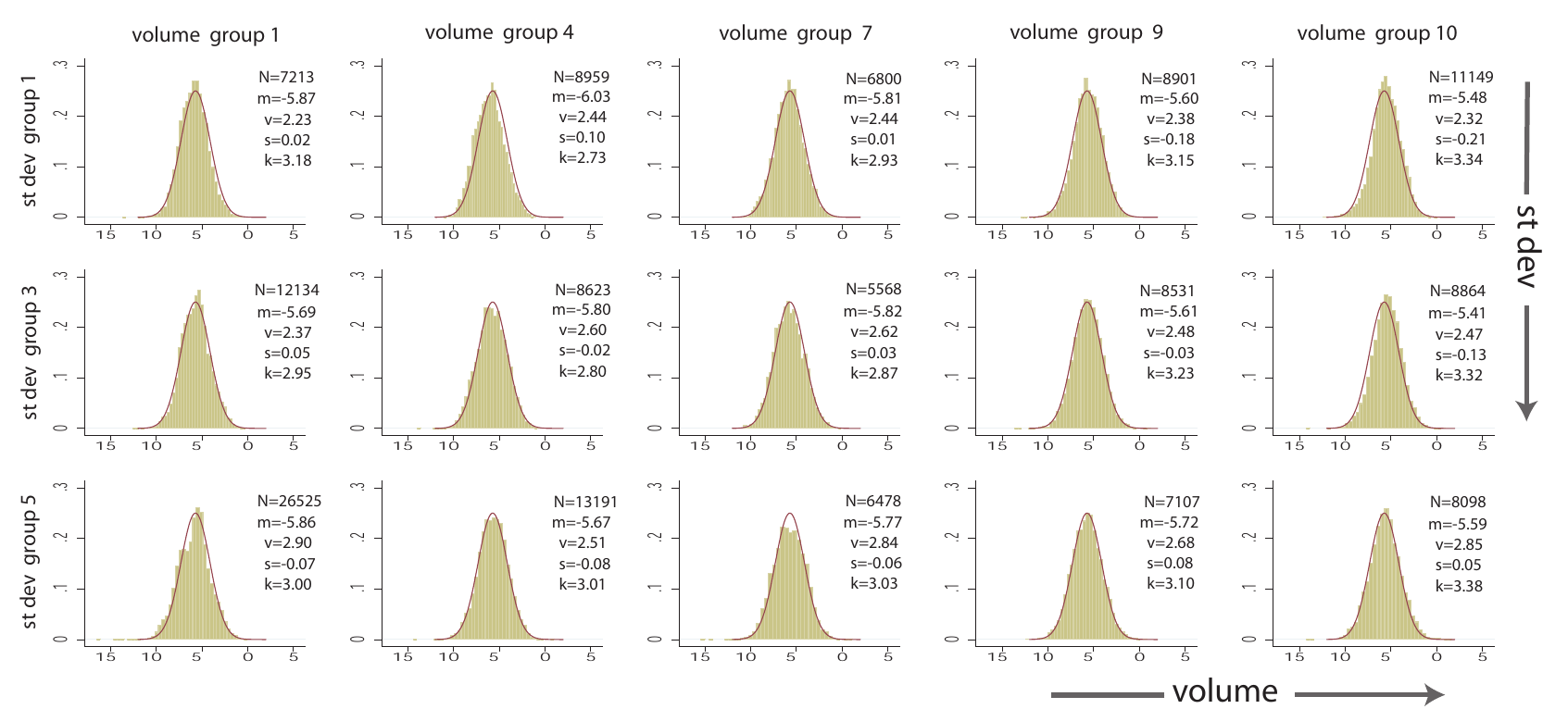
How to read it. Fifteen histograms. The columns are dollar-volume groups 1, 4, 7, 9 and 10 (from quiet stocks to the most active), the rows are volatility groups 1, 3 and 5. Horizontally, the logarithm of order size as a fraction of daily volume plus of the logarithm of relative activity. The same normal curve with mean −5.71 is overlaid on every panel; the figure caption gives its variance as 2.54. In the corner of each panel are the number of orders, the mean (m), variance (v), skewness (s) and kurtosis (k).
What to notice. All fifteen histograms almost coincide with the curve. Means from −6.03 to −5.41, variances from 2.23 to 2.90, skewness from −0.21 to 0.10, kurtosis from 2.73 to 3.38.
The practical takeaway. Raw order sizes in quiet and active stocks differ by tens of times, but after rescaling by activity there is a single distribution. And this distribution is lognormal: the logarithm of size is normal.
Visual similarity does not mean statistical similarity: "Despite the visual similarity, a Kolmogorov-Smirnov test rejects the hypothesis that all fifty empirical distributions are generated from the same normal distribution." The spread of the means across groups is larger than a common distribution allows.
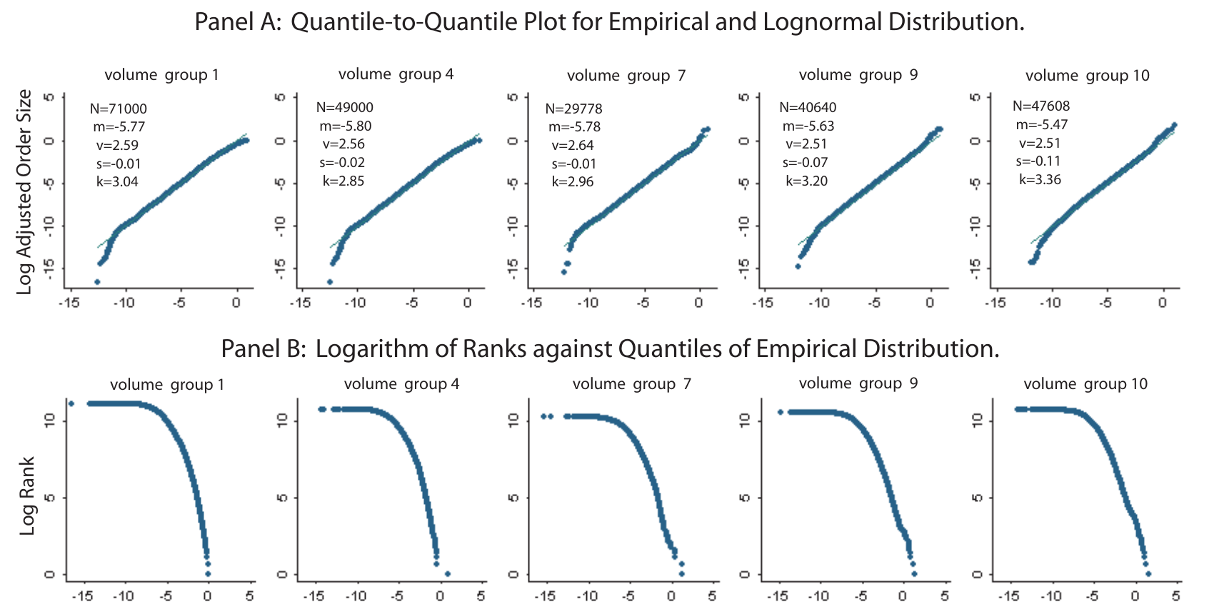
How to read it. Top row (panel A): quantiles of rescaled order size against quantiles of a normal distribution with the same mean and variance, for volume groups 1, 4, 7, 9 and 10. The closer the points are to the straight line, the closer the distribution is to lognormal. Bottom row (panel B): log rank against quantile. Under a lognormal distribution the right tail looks like a parabola here, under a power law like a straight line.
What to notice. The points lie on the line everywhere except at the edges. The smallest orders are smaller than normal; the authors regard them as junk (often one share of a cheap stock, possibly coding errors). The largest orders in quiet stocks have a tail shorter than normal, in active stocks a longer one.
The practical takeaway. The authors explain the short tail in quiet stocks by the disclosure threshold: buying more than 5 % of a company requires filing Form 13D. All orders in the data are below 4.5 % of market capitalization, and the five largest orders in quiet stocks are 2–4 %.
A regression of the log of the order's share of volume on the log of activity gives a slope of −0.62 with a standard error of 0.009 against a predicted −2/3; the hypothesis "is strongly rejected (F = 25.31, p < 0.0001) because the standard error is very small". Across quantiles from the 1st to the 99th the slopes range from −0.61 to −0.65. Buys are closer to −2/3 (−0.63 on NYSE, −0.71 on NASDAQ) than sells (−0.59 on both). The authors explain this by sells liquidating past bets whose size depended on past rather than current activity.
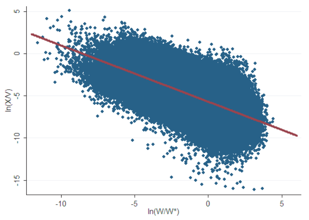
How to read it. Each point is one order, and there are more than 400,000 of them. Horizontally, the log of activity relative to the benchmark stock; vertically, the log of the order's share of daily volume. The red line is not fitted: its slope is fixed at the predicted −2/3, and only the intercept, −5.705, is estimated by least squares.
What to notice. The cloud stretches along the line, and the scatter around it is almost the same across the whole width. The more active the stock, the smaller the share of daily volume that a typical order makes up.
The practical takeaway. The fixed slope of −2/3 explains 31.49 % of the variation in order sizes (). A free slope raises this to 0.3167, and separate exponents for volatility, price, volume and turnover raise it to 0.3229. Almost everything these variables explain at all is explained by activity alone.
What follows from the variance of 2.53. The median order in the benchmark stock equals of daily volume. One standard deviation up means an increase in size by a factor of . From this, by the authors' calculation, bets larger than the median account for 94.41 % of volume, the largest 5.39 % of bets for half of volume, and the largest 0.07 % for half of return variance, if a bet's contribution to variance is proportional to the square of its size. Under stronger assumptions () the benchmark stock has about 85 bets a day, and over a year the 15 largest of 21,420 account for roughly half of return variance. The authors estimate the excess kurtosis of a single bet at this variance at roughly 22,000. Rare giant bets, they suggest, may lie behind crashes such as those of 1929 and 1987 and the flash crash of May 6, 2010.
Lognormal or power law. The authors do not claim the question is settled:
"Whether order size follows a power law or a log-normal distribution is an interesting question for future research."For comparison they cite the size distribution of US mutual funds, also lognormal, with a log variance of about 2.50.
7. The test on costs
Costs are measured by implementation shortfall: the average execution price against the previous close, signed for a buy or a sell. The regression includes the market return on the first day of the transition. The authors warn that if the transitions themselves moved the whole market, this adjustment understates costs: "this adjustment will result in understated transaction costs by measuring only the idiosyncratic component of transaction costs."
First comes a test with no functional form at all: orders are split into 100 bins by rescaled size and into 10 groups by dollar volume, and a separate average cost is estimated for each of the 1,000 cells.
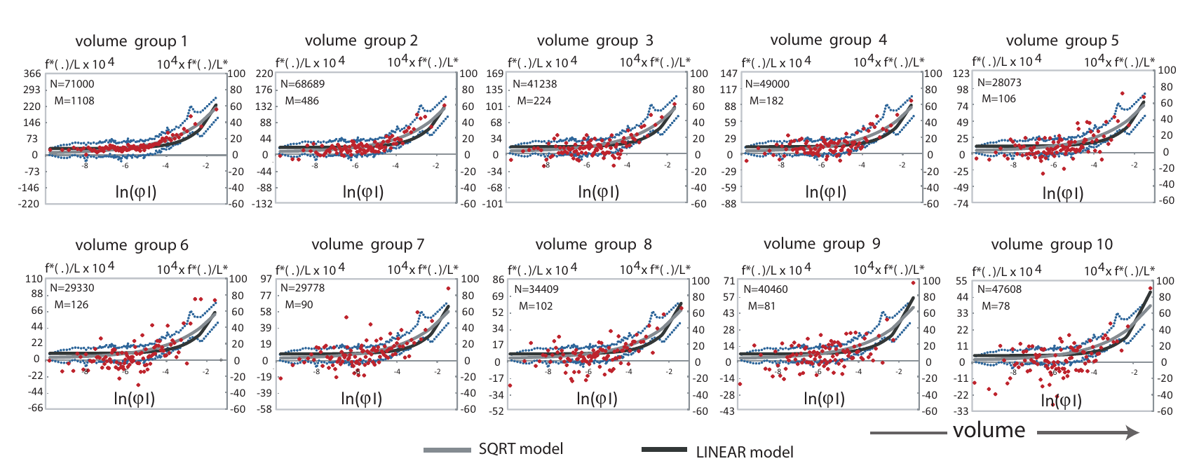
How to read it. Ten panels, one per dollar-volume group, from the quietest stocks (group 1) to the most active (group 10). Horizontally, the log of rescaled order size. The red dots are cost estimates in each of the 100 bins. The left scale gives the group's actual costs in bp, the right scale costs rescaled to the benchmark stock by the invariance formula. The blue dashed line is the 95 % confidence band for the whole sample, the gray line the square-root model, the black line the linear one.
What to notice. The left scales differ: in group 1 costs range from −220 to 366 bp, in group 10 from −33 to 55 bp, seven times narrower. On the right scales, after rescaling, the points in all groups fall along a single band.
The practical takeaway. In group 1 the dots sit inside the band; in group 10 about 11 dots are above it and about 40 below. The authors conclude:
"These patterns suggest that the statistical power of our tests concerning transaction costs comes mostly from low-volume groups."
Then a nonlinear regression with an explicit form: spread plus impact, a power of rescaled size, and separate activity exponents for each part. The results (table 4):
- the activity exponent for impact is (standard error 0.015) against a predicted , which the authors call strong support;
- the exponent for the spread is (standard error 0.050), three standard errors below the prediction; but the spread component itself is significant only at the level of two standard errors, and without it falls from 0.1010 to 0.1006;
- impact curvature (standard error 0.039), closer to the square root (0.5) than to the linear model (1).
An important number for scale: the market return alone explains . The cost models add one to two percentage points to this. With exponents fixed at , the square-root model gives and the linear one 0.0991; free exponents raise it to 0.1010, and twelve free parameters to 0.1016.
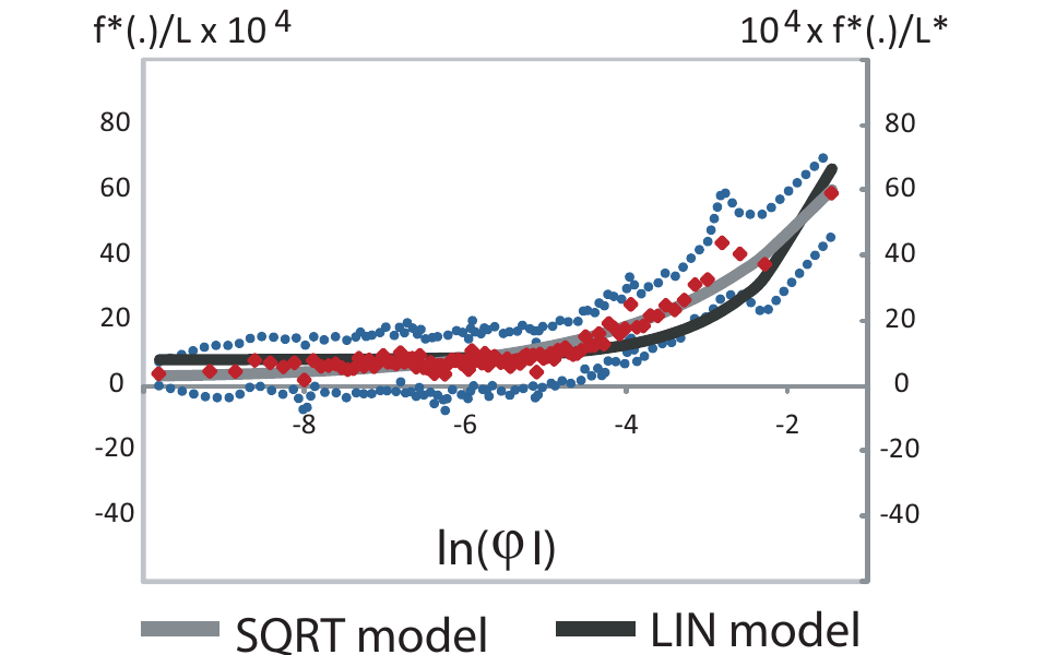
How to read it. The same as figure 4, but for the whole sample at once. The red dots are 100 estimates by size bin, the blue dashed line the confidence band, the gray line the square-root model , the black line the linear one . The horizontal axis is logarithmic and the vertical one is not, so both models look like exponentials.
What to notice. For small orders the cost for the benchmark stock is within a few bp; toward the largest bins it rises to 60-odd bp. The gray line follows the points slightly better, especially in the bins from the 90th to the 99th percentile. The lines cross at the largest percent of orders, and there both fits are equally good.
The practical takeaway. Telling linear from square-root impact apart using the largest orders, where intuitively their predictions should diverge most, does not work here.
The quoted spread is tested separately: the slope of the log of the spread in volatility units on activity is against a predicted , usually rejected statistically, economically close. And an interesting detail: in the cost regression the quoted half-spread explains less than the spread computed from invariance ( 0.0976 against 0.0992), and transitions on average pay only 71 % of the quoted half-spread.
Buys are more expensive than sells in all specifications. The authors link this to the market seeing more information in buys during transitions.
8. Ready-made formulas for calibration
Section 6 of the paper reduces everything to four formulas in which the only stock-specific inputs are dollar volume and volatility. The number of bets per day:
What this is. An estimate of the number of bets per day from trading activity, with and .
Step by step. Multiply daily volatility, price and daily volume in shares. Divide by 800,000. Raise to the power 2/3 and multiply by 85.
An example. The benchmark stock: ratio 1, 85 bets a day. A stock with 8 times the activity: (our example).
Why this matters. An estimate of the “true” market velocity without access to individual decisions. The authors also propose it as the frequency at which data for each asset should be sampled.
Bet size as a fraction of daily volume is distributed as , where is a standard normal variable.
Costs under the square-root model:
What this is. The expected cost of executing an order of shares, as a fraction of its value.
What each symbol means. : the stock's volatility relative to the 2 % benchmark. : activity relative to the benchmark stock (). : order size in percent of daily volume.
Step by step. The first term, the spread: 2.08 bp times activity to the power −1/3. The second, impact: 12.08 bp times the square root of order size in percent of daily volume. Multiply the sum by the volatility ratio.
The authors' example. The benchmark stock, an order of 1 % of daily volume: bp. Under the linear model, bp.
Why this matters. A cost model for any stock from two numbers, dollar volume and volatility. The linear model is built the same way, except that the impact of bp is multiplied by activity to the power and by size in percent of volume without the square root.
The implied spread of the linear model, 16.42 bp, the authors consider close to the quoted one, while the 4.16 bp of the square-root model is probably understated because the constant and the square-root term are hard to tell apart for small orders. If the formulas are applied to markets where the multipliers and are different, the authors require that volume and volatility first be converted into bet volume and bet volatility (footnote 14).
9. What is shaky in the paper
The authors' own caveats
The hypotheses are rejected statistically. "Even though our statistical tests usually reject the invariance hypothesis, the results are economically close to those implied by invariance." The size slope is −0.62 against −2/3, the Kolmogorov–Smirnov test rejects a common distribution, and the spread exponent is −0.49 against −1/3. The paper offers the law as a guide, not as an exact equality.
Market frictions. "Due to market frictions, we do not expect the empirical invariance hypotheses to hold exactly across all assets and all times." And further: "The predictions of invariance may hold most closely when tick size is small, market makers are competitive, and transaction fees and taxes are minimal."
Identifying assumptions. Constant , and for all stocks and periods; if they correlate with activity, the estimates are biased. The authors call these assumptions testable but do not test them in the paper.
Power of the cost tests. Almost all of it comes from quiet stocks; in the group of the most active stocks the estimates are noisy. The authors link this to transitions running on tight calendar deadlines, which for quiet stocks means fast execution in business time.
Execution speed. Invariance assumes that a bet is executed at a “natural” speed. Execution that is too fast may cost more than the formulas give (section 1, “Discussion”).
The market adjustment may understate the costs of large transitions that moved the whole market.
What stands out on reading
The numbers and formulas were not recomputed, and we did not look for discrepancies with the text.
One type of data. Only US common stocks from 2001–2005. The authors call generalization to bonds, currencies, futures and other countries a conjecture. Crypto, futures and currencies are not tested in the paper.
The bet is not observed. All the empirical work rests on the transition order being proportional to a bet. This is an assumption, not a measurement.
Cannot be reproduced. The data are covered by a non-disclosure agreement, and appendix tables A.1–A.5 are absent from the author version we read; the authors refer to an online appendix, which also describes tests on public data.
This is not a strategy. The paper gives a normalization of data and a cost model, not a source of returns.
10. What follows in practice
Slicing data by calendar time is arbitrary. An hour of overnight trading and the hour of a macro data release contain different numbers of decisions. The paper also gives a quantitative hint: the arrival rate of bets is proportional to , so the comparable sampling frequency for two assets differs in the ratio of their activities to the power 2/3.
Share of daily volume compares markets poorly. A limit of “no more than 5 % of daily volume” means different events in an active and in a quiet instrument. The comparable measure is the share of volume multiplied by .
Liquidity helps less than it seems. At the same volatility, a market with 10 times the dollar volume gives percentage costs lower by a factor of about , not 10 (our calculation from the paper's formula). For estimating strategy capacity this is a direct correction.
The number of bets grows faster than their size. When activity grows times, typical bet size grows times. Doubling an instrument's liquidity does not mean the position can be doubled without higher percentage costs.
Average order size is an almost useless statistic. With a lognormal distribution and a log variance of 2.53, about 5 % of bets account for half of volume, and execution risk sits in a few large ones.
Costs are measured more honestly on forced trades. Transitions are valuable because the reason for the trade is unrelated to a price forecast and the order is not canceled in response to the price. Scheduled rebalances, futures rolls and scheduled closes come closest to such an experiment.
The Amihud measure depends on frequency. When comparing the liquidity of assets, it is better to use , which does not depend on time units.
11. Testable ideas
| No. | Idea | Type | Where to compute |
|---|---|---|---|
| 1 | Slice tick data into dollar-volume bars instead of time bars and compare the skewness, kurtosis and autocorrelation of returns | diagnostic | Python |
| 2 | Compute for each instrument and the estimate of the number of bets ; use them as a normalization when comparing instruments and choosing bar size | diagnostic | Python |
| 3 | Convert position limits of the form “no more than X % of daily volume” into invariant units by multiplying the share by , and see how the allowed sizes change across instruments | design change | any |
| 4 | Check on your own executions that percentage costs fall as dollar volume to the power 1/3: the slope in logs should be about −1/3 | audit | Python |
| 5 | Compare the linear and square-root impact models on your own trades, separately for the 90th–99th percentile of size and for the largest 1 % | diagnostic | Python |
| 6 | Select trades unrelated to the signal (rolls, scheduled rebalances, scheduled closes) and measure costs on them separately from signal trades | audit | backtester |
| 7 | Check whether your own order sizes are lognormal after rescaling by , and estimate the log variance; the paper's benchmark is 2.53 | diagnostic | Python |
| 8 | In a backtest, set costs with the paper's square-root model from the instrument's dollar volume and volatility instead of a fixed rate in bp | design change | backtester |