How to read this walk-through. The whole method fits into section 2, “The method in one line”; it can be applied without reading the rest. Section 1 explains why ordinary optimization breaks, and this is the most substantive part of the paper. Section 3 is about why the shrinkage has to be so strong; section 4 is about the link to known methods and can be skipped. Results are in sections 5–7, caveats in section 8. Examples marked “our example” come from our working analysis; we did not recompute the paper's numbers.
The main thesis
Theory says that portfolio optimization should give an investor a lot. In practice, standard mean-variance optimization (MVO, Markowitz, 1952) works so poorly that it is often abandoned. The authors in the introduction: "MVO often produces large and unintuitive bets that perform poorly in practice". It is also known that the simple 1/N portfolio, where capital is split equally, is surprisingly hard to beat with optimization (DeMiguel, Garlappi and Uppal, 2007).
The paper does four things, listed by the authors themselves:
- it finds the “problem portfolios” that make MVO break: these are the least important principal components;
- it proposes a simple fix, enhanced portfolio optimization (EPO), with shrinkage of correlations and a closed-form solution;
- it shows that this fix unifies a number of known methods: the Black–Litterman model, robust optimization, ridge regression from machine learning;
- it tests the fix on data: on trend following in global futures and on industry momentum in US stocks.
The main practical conclusion: the shrinkage of correlations should be chosen by the resulting Sharpe of the portfolio, not by the quality of the matrix estimate, and then it comes out much stronger than is customary.
1. Why standard optimization breaks
What MVO does
The investor gets a signal about the expected excess returns of the assets and an estimate of the covariance matrix . The portfolio that is optimal under the mean-variance criterion (formula 3 of the paper):
What this is. Markowitz's classic solution: the shares of capital in each asset.
What each symbol means. : the vector of capital shares by asset. (“gamma”): risk aversion; the larger it is, the smaller the positions. : the inverse covariance matrix. : the signal; the authors scale it from the start so that it equals the expected excess return.
The calculation in words. The return forecast is divided by risk, taking into account the links between assets. If two assets are almost identical and the forecasts for them differ slightly, the optimizer builds a large “long one, short the other” position, because by its calculation the risk of such a pair is almost zero.
Why this matters. This portfolio gives the highest Sharpe if returns and risk are measured correctly. The authors immediately add that it is sensitive to measurement errors.
Problem portfolios
To find where exactly the error sits, the authors switch to the principal components of the correlation matrix.
What principal components are, in plain terms. They are long-short portfolios that are uncorrelated with one another and ordered by variance. The first component is the riskiest portfolio, usually “the whole market up or down”. The last components are subtle combinations of the form “long one asset, short an almost identical one”, and the data assign them very little risk.
Since the components are uncorrelated, the optimal position in each one is computed separately (formula 5):
What this is. The notional position of the optimal portfolio in principal component number .
What each symbol means. : the expected return of the component. : its variance, its volatility. The first fraction is the component's Sharpe, the second is the leverage needed to bring its volatility to one.
The calculation in words. The desired risk in a component is proportional to its Sharpe, and the notional is in addition inversely proportional to its volatility.
Why this matters. This shows two troubles of the last components. Their risk is selected as the smallest, so estimation errors are more likely to understate it. And the noise in their return estimate is large relative to their risk, so the Sharpe estimate is overstated. The optimizer wants a lot of risk because of the overstated Sharpe and takes on large leverage because of the understated volatility. The authors:
"Further, these two problems exacerbate each other."
In the data this is visible in figure 1 of the paper. It is built on 55 global futures over 1985–2018, sample Global 1; the components are numbered from the most important (1) to the least important (55).
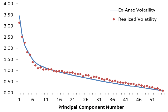
How to read it. The line: the volatility of the component according to the risk model. The dots: the realized volatility.
What to notice. Overall the model works: both decline with the component number. But for the last components the dots are systematically above the line. The authors phrase it cautiously: their risks
"tend to be slightly underestimated".
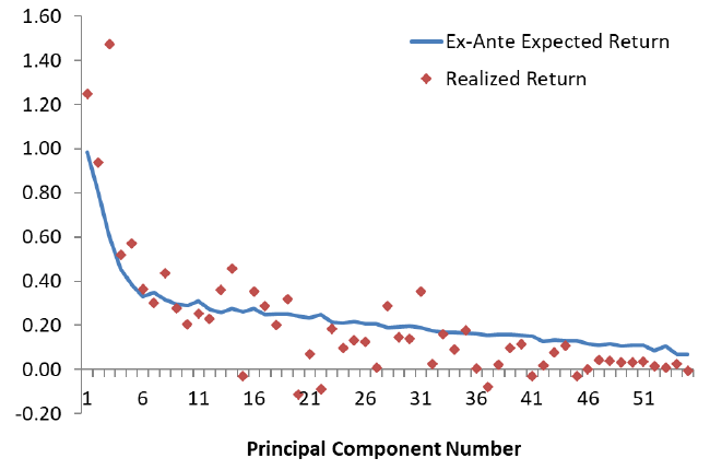
How to read it. The line: the expected return according to the signal; the dots: the realized return.
What to notice. On average both fall with the component number, but the realized return approaches zero faster than the expected one. For the last components the expected return is too high.
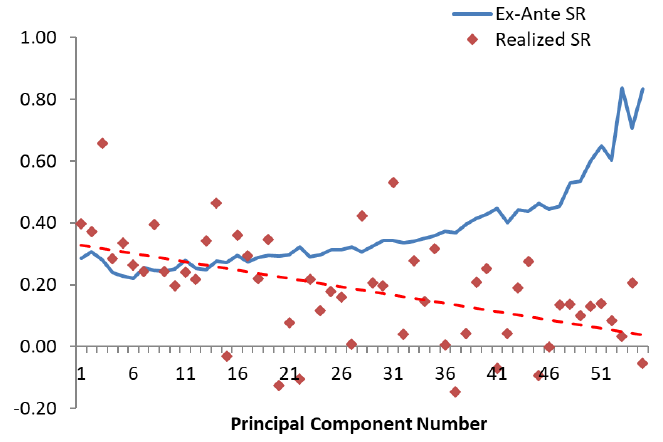
How to read it. The blue line: the expected Sharpe; the dots: the realized one; the red dashed line: the trend of the realized one.
What to notice. The expected Sharpe rises with the component number, from about 0.3 to 0.8, while the realized one falls, along the trend line from about 0.33 to almost zero. The values were read by eye. The authors' explanation: the first components are more likely to reflect real economic factors, while the last ones are unintuitive long-short factors with a low signal-to-noise ratio.
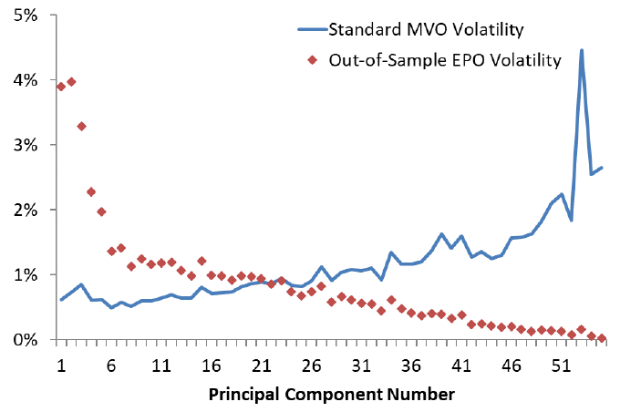
How to read it. The line: how much risk standard MVO actually took in each component; the dots: the same for out-of-sample EPO. Both portfolios are scaled to 10 % annual volatility over the whole period.
What to notice. MVO takes the most risk in the last components, with a peak of about 4.5 % at a component around 53, and less than 1 % in the first ones. EPO is the opposite: about 4 % in the first two and almost nothing in the last ones. The caption of the figure:
"standard MVO invests too heavily in problem portfolios while EPO does not". The notionals in the last components are even larger, because they have to be taken with leverage; the figure does not show this.
2. The method in one line: simple EPO
Since the trouble is that the risk of the last components is understated and that of the first ones overstated, it is natural to pull their variances toward the average. The average variance of the components of a correlation matrix equals one, therefore (formulas 6 and 7):
What this is. The main observation of the paper: shrinking the variances of the principal components toward their average is exactly the same as shrinking the correlation matrix toward the identity matrix.
What each symbol means. : the diagonal matrix of the variances of the principal components. (“omega”): the correlation matrix of the assets. : the identity matrix, ones on the diagonal and zeros off it. (“theta”): the degree of shrinkage, from 0 to 1. A tilde over a letter means “corrected”.
The calculation in words. Take the correlation matrix, multiply all off-diagonal elements by , and leave the diagonal as ones.
Why this matters. By raising the risk of the problem portfolios, we lower their expected Sharpe, and the optimizer stops loading up on them. Shrinking correlations toward zero does this directly.
Simple EPO is assembled like this: the correlation between any pair of assets is replaced with , and ordinary MVO is run on the modified covariance matrix. The authors: "That's it! Note that this is very easy to do." Formally (formulas 15 and 16):
What this is. The simple EPO portfolio.
What each symbol means. (“double-u”): the EPO shrinkage parameter, from 0 to 1. : the estimate of the covariance matrix, possibly already slightly corrected. : the diagonal matrix of variances alone, without correlations. : a mix of the two, that is, the same matrix with correlations multiplied by .
What happens at the extremes. With this is standard MVO. With the correlations are zeroed out, and the solution, according to the authors, essentially amounts to not optimizing at all; it resembles the standard Fama–French factors and even more so portfolios weighted by signal strength. In between, as the authors write, the result is something in the middle, but
"in a way that works surprisingly well".A worked example, our example. The correlation of two assets in the data is 0.90, of a third one with the first 0.30. With they become 0.225 and 0.075. The optimizer no longer sees “almost identical” assets and does not build a large bet on their difference.
Why this matters. The solution is linear in , so the Sharpe of the portfolio does not depend on risk aversion: can be set to one or chosen to hit the desired level of risk.
Shrink first, then optimize. In footnote 2 the authors point out that this is not a simple averaging of two ready-made portfolios. If one computes MVO without shrinkage and the portfolio with full shrinkage and takes a mix of them in any proportion, the result is worse than EPO, especially when MVO behaves badly. The reason, in their words, is that shrinking correlations stabilizes the optimization process itself.
How is chosen. This is an empirical question. Out-of-sample, in each period the authors find the from a finite grid of values that would have given the best Sharpe over the whole history up to that point, and apply it in the next period. The first choice requires at least 15 years of data.
3. Why shrink so strongly
According to the authors, works well in several applications. At the same time, to fix the correlation matrix itself, that is, the errors of the risk model, "we typically need to shrink the correlation matrix only about 5% to 10%". Where does a difference of almost an order of magnitude come from?
The authors' answer: errors in the estimates of expected returns also make shrinking correlations useful, and "these errors may be much larger than the errors in the correlation matrix itself". This is shown in two ways.
A Bayesian model. The investor knows that the signal is noisy: , where is the true expected return and the noise has covariance . The investor's prior belief about is tied to an “anchor” portfolio , the investor's typical portfolio or strategic allocation. The solution (formula 10) looks like MVO in which both the means and the covariances are changed, even though the errors were made only in the means: "errors in expected returns alone lead to the shrinkage of correlations, even when correlations are assumed to be known without error".
Robust optimization. Choose the portfolio that is best under the worst expected return inside an ellipsoid around the signal. The solution (formula 12) coincides exactly with the Bayesian one. According to the authors, this formulation and its solution are new.
If the errors in the signal are assumed to be independent across assets, , the general solution is written in terms of a single parameter (formula 14):
What this is. General EPO with an anchor.
What each symbol means. : the anchor portfolio. (“lambda”): the size of the error in the estimate of expected returns. (“tau”): how strongly the true expected returns vary over time.
The calculation in words. One and the same parameter simultaneously shrinks expected returns toward the anchor and correlations toward zero. With this is MVO, with the anchor portfolio.
Why this matters. The two difficult parameters and disappear, and only their ratio remains. The authors' intuition: the optimal is larger when measurement errors are larger (bad data, illiquidity, a weak predictor) and smaller when the true expected returns vary more.
If the anchor is taken as , that is, the portfolio with full shrinkage, general EPO turns into the simple EPO from section 2.
4. Anchored EPO and the unification of methods
Anchored EPO. Some investors want the portfolio to stay tied to a benchmark: to the index they are measured against, or to a heuristic such as “equal weights across good stocks”. For this the authors give formula 17, where risk aversion is chosen so that the risk of the part built from the signal equals the risk of the anchor. This solves a practical difficulty: the signal is often known only up to scale (for example, a ranking by cheapness), and the “correct units” cannot be plugged into the formula.
Unification. Proposition 3 of the paper lists what the general EPO solution equals in special cases:
- standard MVO, if there is no noise either in the risk estimate or in the signal;
- the anchor portfolio when , as in reverse MVO;
- the Bayesian estimate equivalent to the Black–Litterman model, if the anchor is the market portfolio, the signal is their “view portfolios”, and the covariances are known without error;
- the solution of robust optimization with an ellipsoidal uncertainty set;
- a generalized ridge regression of expected returns on the covariance matrix.
The unification is not all-encompassing, and the authors say so themselves: "EPO obviously does not nest all methods". Methods that improve the covariance matrix itself (Ledoit–Wolf shrinkage, factor models, random matrix theory) are not on this list. On the contrary, the authors write that EPO clearly outperforms them, because it shrinks much more strongly and accounts for noise in both risk and returns.
5. Data and setup
In total there are 11 samples, differing in assets, risk model and signal (table 1 of the paper).
Global 1–3. 55 liquid futures and forwards from the paper by Moskowitz, Ooi and Pedersen (2012): equities, bonds, commodities and nine currency pairs against the US dollar. Cross rates are excluded so that the covariance matrix has full rank. Data from 1970, backtest from 1985 to 2018. Risk model: volatilities from exponentially weighted daily returns with a center of mass of 60 days, correlations from three-day returns with a center of mass of 150 days. Global 2 additionally shrinks correlations by 5 %, Global 3 cleans them with random matrix theory methods.
Equity 1–8. 49 US industry portfolios from Kenneth French's website; in Equity 8 each industry is split into two halves by past 12-month return using CRSP data, 98 assets in total. Data from 1927, backtest from 1942 to 2018. Covariances over windows of 60 months, 40 days or 120 days, correlations shrunk by 5 %. Equity 6 and 7 use anchored EPO with 1/N and as the anchor.
The signal. Everywhere it is the past 12-month return. For futures this is trend following (TSMOM):
What this is. The expected monthly excess return of instrument in month .
What each symbol means. : the volatility estimate of the instrument. (“sign”): if the return over the past 12 months is positive, otherwise . 0.1: the monthly Sharpe of each instrument, assumed constant.
Why this matters. The authors chose the risk aversion so that EPO with full shrinkage coincides exactly with the standard equal-risk trend strategy from the 2012 paper. Then the difference between EPO and the trend shows the contribution of the correlations alone. The 0.1 scale, in their words, does not affect the Sharpe of the resulting portfolio.
For industries the signal is cross-sectional: the past 12-month return of the industry minus the average across all industries, scaled so that the positive and the negative signals each sum to one (formula 18). In Equity 4 and 5 it is additionally multiplied by or .
6. Results on global futures
Sharpes before costs, table 2 of the paper (the caption says it directly: "realized gross Sharpe ratios"):
| Portfolio | Global 1 | Global 2 (5 % shrinkage) | Global 3 (RMT) |
|---|---|---|---|
| Long only, equal notional (1/N) | 0.44 | 0.44 | 0.44 |
| Long only, equal risk (1/σ) | 0.76 | 0.76 | 0.76 |
| Trend, equal notional | 0.74 | 0.74 | 0.74 |
| Trend, equal risk | 1.09 | 1.09 | 1.09 |
| EPO out-of-sample | 1.24 | 1.24 | 1.23 |
| EPO, w = 0 % (ordinary MVO) | 0.87 | 1.08 | 1.02 |
| EPO, w = 25 % | 1.24 | 1.26 | 1.26 |
| EPO, w = 50 % | 1.31 | 1.31 | 1.32 |
| EPO, w = 75 % | 1.32 | 1.31 | 1.32 |
| EPO, w = 90 % | 1.26 | 1.26 | 1.26 |
| EPO, w = 100 % (anchor) | 1.09 | 1.09 | 1.09 |
How to read it. The equal-risk trend is already a strong benchmark: according to the authors, it does part of the optimizer's job by taking into account both expected returns and the differences in volatility; the only thing it does not use is correlations. The authors:
"Nevertheless, the out-of-sample EPO significantly outperforms TSMOM by 14%".What matters. The gain from 1.09 to 1.24 is obtained on the same signal and the same instruments; only the way of turning signals into weights changed. Standard MVO (0.87 in Global 1) is worse than the simple equal-risk trend. The rows with a fixed are computed in-sample: picking the best with hindsight is impossible in real time, and the authors point this out.
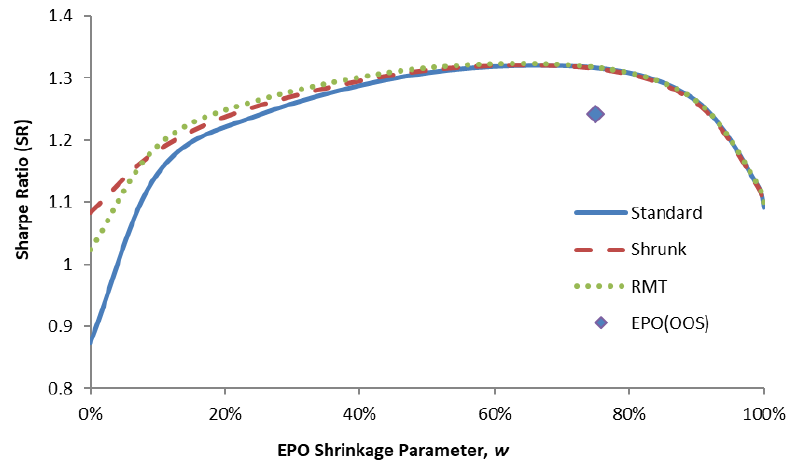
How to read it. Horizontally, from 0 to 100 %; vertically, the Sharpe. Three curves for three risk models (standard, shrunk by 5 %, cleaned with RMT), a diamond for out-of-sample EPO.
What to notice. On the left the curves diverge: improving the correlation matrix raises the Sharpe of MVO from 0.87 to 1.02–1.08. Near the maximum they merge. The authors:
"improving the correlation matrix is important for standard MVO, but has little effect when we subsequently shrink the correlation by a large factor". The curve is flat over a wide range: according to the table, from 25 to 90 % the Sharpe is from 1.24 to 1.32.
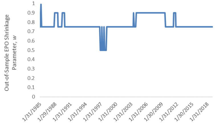
How to read it. Horizontally, time from 1985 to 2018; vertically, the chosen for each month.
What to notice. Most of the time the parameter sits at 0.75, a long stretch from about 2004 to 2010 at 0.9, short dips to 0.5 around 1997, and at the very beginning 1. The authors write that at first the process picks a lower shrinkage and needs time to arrive at the best value; this is why out-of-sample EPO is slightly below the in-sample maximum.
Alpha (table 3). All series are scaled to 10 % annual volatility. The regression of EPO on the equal-risk trend gives an alpha of 2.48 % per year (t = 3.36) with an of 83 % and an information ratio of 0.60. With the long portfolio added, the alpha is 2.17 % (t = 2.92); with the long portfolio and trends for each of the four asset classes, 2.11 % (t = 2.93). The reverse regression, of the trend on EPO, gives an insignificant alpha of −0.43 % (t = −0.57).
Leverage and turnover (table 4, Global 2, at 10 % volatility).
| Portfolio | Gross leverage | Annual turnover, % of average leverage |
|---|---|---|
| Trend, equal risk (anchor, w = 100 %) | 358 % | 163 % |
| EPO out-of-sample | 457 % | 254 % |
| EPO, w = 90 % | 424 % | 208 % |
| EPO, w = 75 % | 479 % | 263 % |
| EPO, w = 0 % (ordinary MVO) | 991 % | 546 % |
The weaker the shrinkage, the larger the leverage and the turnover. The authors conclude that with a suitable the portfolios are implementable, and state directly: "While the EPO method shown here abstracts from transaction costs". Accounting for costs inside the optimization could, in their words, reduce turnover; this is left for future work.
7. Results on US industries
Table 5 of the paper, Sharpes before costs, 1942–2018:
| Portfolio | Range across Equity 1–8 |
|---|---|
| 1/N, equal notional | 0.57–0.59 |
| Standard industry momentum (INDMOM) | 0.63–0.67 |
| MVO without shrinkage of correlations | from −0.02 to 0.92 |
| EPO out-of-sample | 0.66–0.99 |
How to read it. Out-of-sample EPO beats 1/N, industry momentum and MVO in all eight variants. It is close to the best in-sample value with a fixed everywhere,
"except for Equity 2": there it is 0.72 out-of-sample against 0.93 in-sample. MVO without shrinkage is extremely unstable: from 0.92 in Equity 3 to −0.02 in Equity 2.Comparison with factors. According to footnote 22, from 1963 to 2018 the five Fama–French factors give Sharpes from 0.27 to 0.49, and their equal-weighted mix 0.93. All variants of out-of-sample EPO are above each individual factor, and the best ones are above the mix too, even though EPO relies only on industry returns.
Alpha (table 6). The regression of out-of-sample EPO on industry momentum and the five Fama–French factors, 1963–2018, everything at 10 % volatility. The alpha is positive everywhere, from 1.07 to 8.09 % per year. It is significant at the 5 % level everywhere except Equity 6, where "the t-statistic of 1.80 is only significant at a 10% level". In Equity 2–4 the t-statistic is above 6. The authors explain the weakness of Equity 6 by the anchor there being the long 1/N portfolio: hence a market loading of 0.85 and a conflict between stabilization and a tilt toward a portfolio that does not use the signal.
8. What is shaky in the paper
Caveats from the authors themselves
There are no costs. All Sharpes are gross, and the optimization does not account for costs. Meanwhile out-of-sample EPO trades with more leverage and turnover than the equal-risk trend: 457 % against 358 % and 254 % against 163 % per year.
The best in-sample is unattainable. The table rows with a fixed are hindsight. The only fair comparison is with the “out-of-sample” row, and on futures it is 0.07–0.09 below the in-sample maximum (our calculation from table 2).
The conflict of interest is disclosed. In the first footnote: AQR "may or may not apply similar investment techniques or methods of analysis as described herein". The trend strategy the method is tested on is built from a paper co-authored by one of the authors.
The signal is simple on purpose. Everywhere it is the past 12-month return. The authors write that the method is general and leave other predictors to future research.
The unification is not all-encompassing. EPO does not include all methods; this is said directly.
What is visible on reading but not discussed in the paper
Our working analysis has no discrepancies confirmed by a quotation, so discrepancies is zero. We did not recompute the numbers.
The data for the main result are not public. The series for the 55 futures were assembled by the authors and not published; Equity 8 relies on the licensed CRSP database. The industry portfolios of Equity 1–7 and the Fama–French factors are open, and this part can be replicated.
Choosing is itself a form of fitting, albeit an honest one. The grid of values is finite, and the selection is by past Sharpe. In figure 2 the parameter sits almost all the time at one of three values (0.5, 0.75, 0.9). The paper does not show how sensitive the result is to the grid step.
Momentum only. Both tests are on momentum signals, where the signal is directly linked to past returns. For signals with a different error structure, the size of the best shrinkage may be different; by the paper's own logic it depends on the ratio of the noise in the signal to the variation of the true returns.
9. What follows in practice
The problem of optimization is not the optimization but the trust placed in subtle combinations. The choice is not between “optimize” and “1/N” but about how much to believe the last principal components.
The fix costs one line. Multiply the off-diagonal elements of the correlation matrix by and run the same optimization. No libraries or complex computations are needed for this.
Choose the shrinkage by the resulting out-of-sample Sharpe, not by the quality of the matrix estimate. These are two different criteria, and in the paper they give answers of about 75 % and about 5–10 %.
Near the optimum the result is insensitive to . On futures the Sharpe is from 1.24 to 1.32 for from 25 to 90 %. This means that the parameter itself does not become a new source of overfitting, but also that there is no need to search for the exact value.
Shrink first, then optimize. A mix of a ready-made MVO portfolio and a portfolio without correlations, according to the authors' footnote, works worse in any proportion.
Report leverage and turnover next to the Sharpe. Less shrinkage quickly increases both: MVO without shrinkage has leverage of 991 % and turnover of 546 % against 358 % and 163 % for the anchor, that is, about 2.8 and 3.3 times more (our calculation from table 4). The gain in gross Sharpe has to be weighed against the cost of this turnover.
The anchor as a mechanism of caution. Anchored EPO turns optimization into a correction to an understandable portfolio (1/N, equal risk, an index), not a replacement for it.
10. Testable ideas
| No. | Idea | Type | Where to compute |
|---|---|---|---|
| 1 | Before optimizing weights, multiply the off-diagonal correlations by ; choose out-of-sample by past Sharpe on an expanding window from a grid of values | design change | Python |
| 2 | Plot the “Sharpe against ” curve from 0 to 1: is there an interior maximum and how flat is the curve around it | diagnostic | Python |
| 3 | Decompose your own set of assets or strategies into principal components and compare expected and realized volatility, return and Sharpe by component number, as in figure 1 | diagnostic | Python |
| 4 | Compare the degree of shrinkage chosen by the quality of the covariance matrix estimate with the degree chosen by the out-of-sample Sharpe of the portfolio | audit | Python |
| 5 | Report gross leverage and annual turnover next to the Sharpe for each , and compute the Sharpe after your own costs | acceptance metric | backtester |
| 6 | Anchored EPO with your current heuristic weights (equal notional or equal risk) as the anchor: see what corrections the optimization proposes | design change | Python |
| 7 | On unchanged signals, break the gain down by stages: equal notional, equal risk, out-of-sample EPO | diagnostic | backtester |
| 8 | Check footnote 2 on your own data: compare EPO with mixes of the ready-made MVO and full-shrinkage portfolios in different proportions | audit | Python |