Dynamic signal weighting: when it adds value and when it does not

How to read this walk-through. The paper's main conclusion fits in one sentence: changing signal weights by regime makes sense when the signals diversify each other poorly, not when the regime is easy to recognize. That is the section “The main thesis” and section 4. Sections 1–3 show where the conclusion comes from: the formulas are explained symbol by symbol, but they can be skipped. The numbers in examples marked “our example” come from our working notes; we did not recompute the paper's numbers.

The main thesis

A strategy can be built from several signals, say from value (cheapness) and momentum (the strength of past gains). There are two ways to mix them:

static: the weights are set once and for all;
dynamic: the weights depend on the market or economic regime. The author notes that this is the same thing as factor timing or style rotation.

Intuition suggests that if we can recognize the regime and know that momentum works better in regime A and value in regime B, the dynamic approach should win. The author shows that this is not enough. In the abstract: "But interestingly, this is not a sufficient condition." Two conditions are needed at once:

the behavior of the signals really differs from regime to regime;
the returns of the signals are strongly correlated with each other.

The second condition is not obvious. The author's logic is this: if the signals are weakly or negatively correlated, the static mix is already well diversified, and its quality rests on diversification, not on guessing the regime. By shifting the weights we lose diversification. The conclusion states this cautiously: "Usually, the more diversified the static model, the lower the gain in contextual modeling." And further: "the results suggest that the first-best solution is to build well diversified strategies". If that is impossible, contextual modeling, according to the author, can become a valuable alternative, but "this alternative is risky".

The paper deliberately simplifies the picture, and the author says so directly: "This is why we simplify reality." Two signals, unconstrained portfolios, constant correlation, a precisely known regime. The goal is to make the conditions under which dynamics helps visible in the most transparent form.

1. How the model is built

The forecast as a mix of signals

\alpha = w_1 z_1 + w_2 z_2

What this is. The starting point of any multifactor model: the return forecast is assembled as a weighted sum of signals.

What each symbol means.

$\alpha$ (alpha): a column of $N$ numbers, one for each asset in the universe. This is our return forecast for each asset.

$z_1, z_2$ (zee one, zee two): also columns of $N$ numbers, the values of the first and second signal for each asset. For example, $z_1$ shows how cheap a stock is, and $z_2$ how much it has risen over the year.

$w_1, w_2$ (double-u): the weights of the signals, two ordinary numbers. These are what we choose.

Step by step, our example. Three stocks. The cheapness signal $z_1 = (2,\ 0,\ -1)$ , the momentum signal $z_2 = (-1,\ 1,\ 1)$ , the weights $w_1 = 0.6$ and $w_2 = 0.4$ . The first stock: $0.6 \cdot 2 + 0.4 \cdot (-1) = 0.8$ . The second: $0 + 0.4 = 0.4$ . The third: $-0.6 + 0.4 = -0.2$ . We buy the first one most heavily and sell the third.

Why this matters. The weights are exactly what the static and dynamic approaches disagree about. The author notes in a footnote that the weights do not have to sum to one: their overall size is set by the strategy's target volatility.

h_k = \Sigma^{-1} z_k

What this is. The step from a signal to a portfolio: scores for the assets turn into concrete positions.

What each symbol means.

$\Sigma$ (capital sigma): the covariance matrix of asset returns, an $N \times N$ table. The diagonal holds the variances of individual assets; off the diagonal are the joint movements of pairs.

$\Sigma^{-1}$ : the inverse matrix. For an ordinary number, the inverse of 5 is 1/5; for a matrix the idea is the same, only the role of “one” is played by the matrix with ones on the diagonal.

$h_k$ : the positions of the portfolio built from signal number $k$ .

In words. Multiplying by $\Sigma^{-1}$ is like dividing the forecast by risk, only taking the links between assets into account. A volatile asset gets a smaller position. Two very similar assets do not both get full positions, because that would be one bet of double size.

Why this matters. From here on the author works not with the signals but with these “signal portfolios”: the return of the strategy turns out to be a weighted sum of their returns.

The signals are normalized so that each signal portfolio has unit volatility: $z_k^{\top}\Sigma^{-1}z_k = 1$ . Then the expected return of the whole strategy is written very simply:

r_p = w_1\, IR_1 + w_2\, IR_2

What this is. The expected return of a strategy built from two signals.

What each symbol means. $IR_k$ (information ratio, “eye-ar”): the expected return of the signal portfolio divided by its volatility. In meaning it is the same as the Sharpe ratio, only for a long-short portfolio without the market component. Since the volatility of each signal portfolio equals one, its contribution to return equals its $IR$ multiplied by its weight.

Why this matters. The problem “how to mix signals” reduces to the problem “how to split risk between two bets of known quality”.

Optimal weights

Without loss of generality the author sets the strategy's target risk to one and looks for the weights that give the highest return:

\max_{w_1,\, w_2}\ r_p \quad \text{subject to} \quad w_1^2 + w_2^2 + 2\rho\, w_1 w_2 = 1

What this is. “Maximize return at a fixed risk.” The $\max$ symbol with a subscript reads “choose the $w_1$ and $w_2$ at which the expression is largest”.

What the constraint means. The left side is the squared volatility of the mix of two signal portfolios. $\rho$ (rho): the correlation of their returns. The author notes: "For the sake of simplicity, this correlation is assumed to be constant over time."

Why the cross term matters. At $\rho = 0$ the risks of the two bets add up “by Pythagoras”, and the total risk is less than the sum. At $\rho = 1$ the signals duplicate each other, and there is no diversification. At $\rho = -1$ the bets cancel each other out.

w_1^{*} = \frac{IR_1 - \rho\, IR_2}{\lambda\,(1-\rho^2)}, \qquad w_2^{*} = \frac{IR_2 - \rho\, IR_1}{\lambda\,(1-\rho^2)}

What this is. The solution of the problem, formula (5) of the paper.

What each symbol means. $\lambda$ (lambda): the Lagrange multiplier, a technical coefficient that adjusts the overall size of the weights to the given risk. The asterisk means “optimal value”.

In words. In the numerator, a signal's weight equals its own quality minus the neighbor's quality multiplied by the correlation. A signal is penalized for repeating its neighbor.

A worked example, our example. $IR_1 = 0.6$ , $IR_2 = 0.4$ . At $\rho = 0$ the numerators are 0.6 and 0.4: the weights are proportional to quality. At $\rho = 0.8$ the numerators are $0.6 - 0.8 \cdot 0.4 = 0.28$ and $0.4 - 0.8 \cdot 0.6 = -0.08$ : the second signal gets a negative weight and is needed only as a hedge for the first.

Why this matters. This shows when the second signal is redundant as a standalone bet: when $IR_2 - \rho\, IR_1 < 0$ .

\lambda = IR^{*} = \frac{\sqrt{IR_1^2 + IR_2^2 - 2\rho\, IR_1 IR_2}}{\sqrt{1-\rho^2}}

What this is. The quality of the optimal mix, formula (6). The Lagrange multiplier turns out to equal the best achievable $IR$ .

A worked example, our example. $IR_1 = 0.6$ , $IR_2 = 0.4$ . At $\rho = 0$ : $\sqrt{0.52} \approx 0.72$ , better than either signal alone. At $\rho = -0.5$ : $\sqrt{0.76/0.75} \approx 1.01$ . At $\rho = 0.8$ : $\sqrt{0.136/0.36} \approx 0.61$ , almost nothing beyond the best signal.

Why this matters. The value of the second signal is determined not only by its quality but also by how unlike the first one it is.

2. Static against dynamic: how far apart the weights are

The author introduces $J$ regimes (“contexts”) numbered $j$ . This can be a market, economic or any other context. The proposal is to compare two ratios:

b = \frac{IR_2}{IR_1}, \qquad b_j = \frac{IR_{2j}}{IR_{1j}}

What this is. $b$ : how many times better the second signal is than the first on average over the whole history. $b_j$ : the same within regime $j$ .

The author's assumption. The expected $IR$ s of both signals are always strictly positive, so $b$ and $b_j$ are positive too. A footnote clarifies where these numbers come from in practice: for example, as historical averages over the whole history and over the periods of regime $j$ .

The key point the author singles out. What matters is the relative quality of the signals, not the absolute one. If in a crisis both signals become twice as bad, then $b_j = b$ , and there is no reason to change the weights. The author stresses that this is especially important for strategies with a constant target volatility.

The static approach keeps the optimal weights constant. The dynamic one takes, in each regime, the weights that are optimal for that regime; the author notes in a footnote that the current regime is taken as known, uniquely defined and unchanging over the investment horizon: "supposing that this context does not change on the investment horizon considered".

The weight differences $\Delta w_{1j}$ and $\Delta w_{2j}$ (dynamic minus static) are written out in formula (7) of the paper; they depend only on $b$ , $b_j$ and $\rho$ . The author measures the distance between the two models as follows:

d_j(b, b_j, \rho) = \sqrt{\frac{\Delta w_{1j}^2 + \Delta w_{2j}^2 + \Delta w_{1j}\,\Delta w_{2j}}{2}}

What this is. How much the weights of the dynamic model in regime $j$ differ from the static ones. The author calls this the root-mean-square difference of the weights and refers to Sorensen and coauthors (2005).

What each symbol means. $\Delta$ (delta): a difference. $\Delta w_{1j}$ : the weight of the first signal in regime $j$ minus its constant weight.

Why this matters. This is an intermediate gauge. If the distance is small, the two models almost coincide, and there is nothing to argue about.

What the author proves. In $b_j$ the distance has the shape of the letter U with a zero at $b_j = b$ : the more a regime changes the relative quality of the signals, the further apart the models move. In $\rho$ the behavior depends on the case. If the leader changes in the regime (on average one signal is better, but in the regime the other one is, that is, $b_j < 1 \le b$ or $b \le 1 < b_j$ ), the distance grows monotonically as the correlation rises. Otherwise it has the shape of an inverted U with a maximum at a positive correlation.

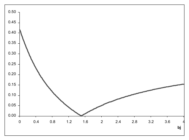
Curve of the distance between the models as a function of b_j: zero at b_j = 1.5, rising on both sides — Figure 1 of the paper (Exhibit 1): distance between the models and the relative quality of the signals, b = 1.5, ρ = −0.2

How to read it. Horizontally, $b_j$ from 0 to 4; vertically, the distance $d_j$ . Computed by the paper's formula at $b = 1.5$ and $\rho = -0.2$ ; according to the author, this value of the correlation "is roughly in line with the level of valuation and momentum performance correlation found in equity universes".

What to notice. The curve touches zero exactly at $b_j = 1.5$ , where the regime does not differ from the average at all. To the left it rises more steeply: by eye about 0.42 at $b_j = 0$ against roughly 0.15 at $b_j = 4$ .

Why the correlation affects the result so strongly can be seen from the ratio of the weights:

\frac{w_1}{w_2} = \frac{1 - \rho\, b}{b - \rho}, \qquad \frac{w_{1j}}{w_{2j}} = \frac{1 - \rho\, b_j}{b_j - \rho}

What this is. The ratio of the optimal weights, formula (9): on the left the static one, on the right the one in regime $j$ .

Step by step. Substitute $\rho = -1$ : this gives $\frac{1+b}{b+1} = 1$ , and the same for $b_j$ . That is, as the correlation tends to $-1$ , the optimal weights tend to become equal, however much the quality of the signals differs.

Why. When two bets cancel each other's risk, each is valuable above all as insurance for the other. The author writes that in this case a noticeable change in the weights hurts the strategy, because the risk grows more than the gain. That is also why the distance between the models is small.

Why this matters. The author calls this result central to explaining when dynamics adds value.

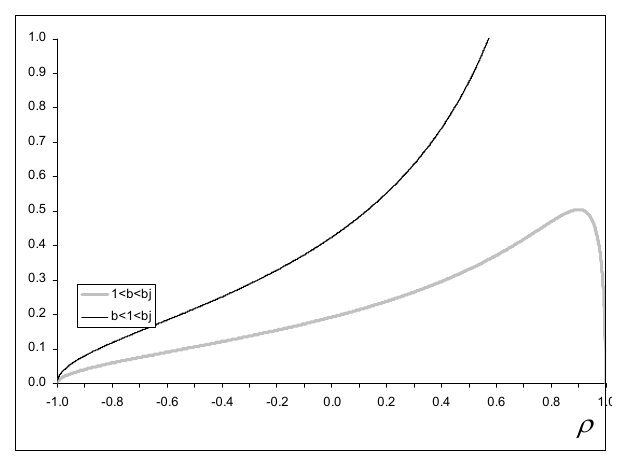
Two curves of the distance between the models as a function of the signal correlation from −1 to 1 — Figure 2 of the paper (Exhibit 2): distance between the models and the signal correlation

How to read it. Horizontally, the correlation $\rho$ from $-1$ to $1$ ; vertically, the distance. The black curve is labeled b<1<bj (the leader changes), the gray one 1<b<bj (the leader stays the same).

What to notice. At the left edge both curves are pressed down to zero: with a strongly negative correlation the models are almost indistinguishable. The black curve rises monotonically and goes off the top of the chart. The gray one reaches a maximum of about 0.5 at a high correlation and then falls. The text says that at $b = 1.5$ and $b_j = 2$ the maximum is reached at $\rho = 0.94$ ; the note under the figure itself gives $b_j = 4$ (see section 5).

3. The main result: how much static loses

The expected quality of the strategy in regime $j$ with dynamic weights (formula 10 of the paper):

IR_j^{D} = IR_{1j}\sqrt{\frac{1 + b_j\,(b_j - 2\rho)}{1-\rho^2}}

and with static weights (formula 12):

IR_j^{S} = IR_{1j}\,\frac{1 + b\,b_j - \rho\,(b_j + b)}{\sqrt{(1-\rho^2)\,\bigl[1 + b\,(b - 2\rho)\bigr]}}

What this is. The letter $D$ stands for dynamic, $S$ for static. Both formulas are obtained by substituting the optimal weights into the expression for $IR$ . There is no need to compute them by hand: what matters is their ratio.

L_j(b, b_j, \rho) = \frac{IR_j^{S}}{IR_j^{D}} = \frac{1 + b\,b_j - \rho\,(b_j + b)}{\sqrt{\bigl[1 + b\,(b-2\rho)\bigr]\bigl[1 + b_j\,(b_j-2\rho)\bigr]}}

What this is. The main formula of the paper, formula (13): what share of the dynamic model's expected quality the static one keeps in regime $j$ .

What each symbol means. $L$ from “loss”: the relative quality of static. $b$ , $b_j$ , $\rho$ are the same as above. $IR_{1j}$ cancels in the ratio, so $L_j$ does not depend on the absolute quality of the signals.

In words. Take three numbers: the average ratio of the signals' quality, the same ratio in the regime, and the correlation. Compute the numerator and the two factors in the denominator, take the square root, divide. $L_j = 1$ means dynamics gives nothing; $L_j = 0.9$ means static loses 10 % of quality.

A worked example on the paper's numbers. Figures 3 and 4 below are built from exactly this formula at $b = 1.5$ , $\rho = -0.2$ and at $b = 0.5$ or $1.5$ , $b_j = 4$ .

What is proved about this quantity.

$L_j$ is at most one: "the ex ante -i.e. based on expectations- value added of the dynamic approach is always positive". A footnote immediately adds a caveat: "This is not necessarily the case ex post."

$L_j$ depends only on three numbers, $b$ , $b_j$ , $\rho$ .

In $b_j$ the function rises up to $b_j = b$ and falls after it: the further a regime moves relative quality away from the average, the more static loses.

In $\rho$ : if the leader changes in the regime, $L_j$ decreases monotonically as the correlation rises, and the benefit of dynamics grows. Otherwise the shape is a U, and the greatest benefit is reached at a positive correlation.

Why this matters. This is a ready-made calculator for the decision “build a regime layer or not”: three numbers, and the formula says how much expected quality we lose by staying with constant weights. But only expected quality, and only with a precisely known regime.

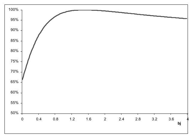
Dome of the relative quality of static as a function of b_j, maximum of about 100 % around b_j = b — Figure 3 of the paper (Exhibit 3): expected relative quality of static and the relative quality of the signals, b = 1.5, ρ = −0.2

How to read it. Horizontally, $b_j$ ; vertically, $L_j$ in percent. Computed by formula (13) at $b = 1.5$ , $\rho = -0.2$ .

What to notice. The curve is near 100 % for $b_j$ from about 1.2 to 1.8 and falls off on both sides, but not symmetrically. By eye: about 66 % as $b_j \to 0$ and about 96 % at $b_j = 4$ . So even with a negative correlation, static can lose a noticeable share of quality if the regime shifts the balance of the signals strongly in one direction.

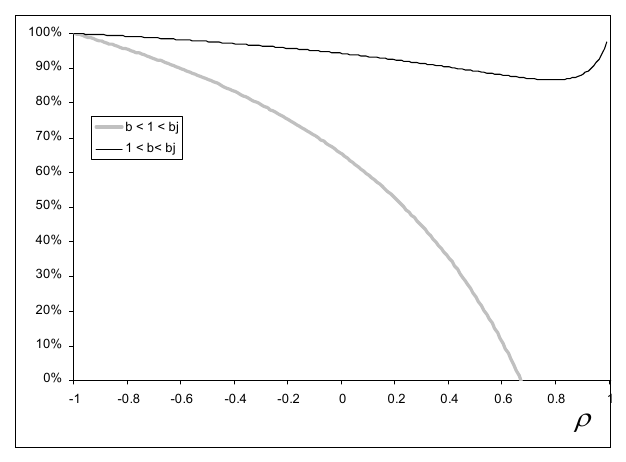
Two curves of the relative quality of static as a function of the signal correlation — Figure 4 of the paper (Exhibit 4): expected relative quality of static and the signal correlation

How to read it. Horizontally, the correlation; vertically, $L_j$ . The gray curve is b < 1 < bj (the leader changes, $b = 0.5$ , $b_j = 4$ ), the black one 1 < b< bj (the leader stays the same, $b = 1.5$ , $b_j = 4$ ).

What to notice. At the left edge both curves are at 100 %: with a correlation of about $-1$ static loses nothing. The black curve is almost horizontal and dips to roughly 87 % at a correlation of about 0.8, then comes back up. The gray one falls all the way: about 65 % at zero correlation and down to zero at about $\rho \approx 0.67$ . The values are read off by eye.

The practical takeaway. The gain from dynamics grows with the correlation, and when the leader changes in the regime it can be large already at moderate correlations.

Finally, the author looks for the correlation at which dynamics helps most:

\hat\rho(b, b_j) = \arg\min_{\rho \in [-1,\,1]} L_j(b, b_j, \rho)

What this is. The $\arg\min$ symbol reads “the value of the argument at which the function is smallest”. The smallest $L_j$ means the greatest benefit from dynamics. The hat over $\rho$ (“rho hat”) marks the value found.

The author's answer. For reasonable values, when $b$ and $b_j$ are not both very large or both very small, this correlation is fairly high, and when the leader changes it equals 1. On average over all pairs of $b$ and $b_j$ from 0 to 10 in steps of 0.1 (except $b = b_j$ , where $L_j = 1$ at any correlation), the result was "around 0.57, which is indeed relatively strong".

Why this matters. This is not a threshold beyond which dynamics pays off, but the average location of the maximum benefit. It says that dynamic weighting is, by its very construction, designed for signals that diversify each other poorly.

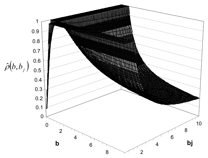
Three-dimensional surface of the correlation that maximizes the benefit of dynamics, along axes b and b_j from 0 to 10 — Figure 5 of the paper (Exhibit 5): the signal correlation at which the benefit of the dynamic approach is greatest

How to read it. Two horizontal axes, $b$ and $b_j$ , from 0 to 10; vertically, $\hat\rho$ from 0 to 1.

What to notice. Along the edges where the leader changes, the surface sits at the level of 1. It drops in the corner where both ratios are large and at the very edge where both are small. Over most of the area the values are high.

4. The author's two conditions

In the section on practical implications, the author states two conditions under which the benefit of dynamics is significant.

Condition 1: the regime must really separate the relative quality of the signals, that is, $b_j$ differs noticeably from $b$ . This shapes the choice of a regime indicator: it should be judged by its ability to pull the quality of the signals apart relative to each other, not by its ability to explain the market in general. The author adds that this condition is "necessary but not sufficient".

Condition 2: the correlation of the signals' returns must be high. The author's general rule: the worse diversified the static model, the larger the gain from dynamics. With a high correlation the benefit of diversification is small, and the quality of the strategy is mostly determined by the ability to bet on the right style at the right time. With a weak or negative correlation the expected quality of dynamics is, according to the author, "only slightly higher than that of the static model". And the final statement of the section: "if the static model is already well diversified, the contextual modeling is likely to add little value".

5. What is shaky in the paper

The author's own caveats

The expected benefit is not the realized one. The conclusion lists what the realized result depends on besides the two conditions: uncertainty in identifying the regime, uncertainty in estimating the relative quality of the signals by regime, and the extra costs of the turnover created by switching models. The author ends with: "The analysis of these effects warrants further research." None of this is computed in the paper itself.

The regime is known precisely and does not change over the horizon. This is stated in footnote 3: the dynamic approach here takes the current context as given and relies on the assumption that it can be characterized unambiguously.

The correlation is constant. This is given as a simplification. Yet the paper itself is about signal parameters changing from regime to regime; whether the correlation stays constant across regimes has to be checked separately.

The expected $IR$ s of both signals are strictly positive. This simplifies the exposition; the case where one of the signals loses money on average in a regime is not covered.

Only two signals and unconstrained portfolios. A generalization to more signals is not considered in the paper.

What we noticed while reading

Our working notes contain no discrepancies confirmed by a quote, so discrepancies is zero. We did not recompute the numbers. Three things stood out while reading the PDF; they do not affect the conclusion and are not counted.

The note to figure 2 disagrees with the text. In the text the curves of figure 2 are described at $b = 0.5$ , $b_j = 2$ and $b = 1.5$ , $b_j = 2$ , with a maximum "for ρ = 0.94". The note under the figure gives $b_j = 4$ for both cases, and the note under figure 4 also gives $b_j = 4$ . Which value is correct for figure 2 cannot be established from the text.

A typo in the denominator of formula (11). It has $w_1^2$ twice instead of $w_1^2 + w_2^2$ ; in the next line the author uses the correct expression for volatility, so this is a typesetting error.

The general statement is stronger than the figures. The sentence saying that with a weak or negative correlation dynamics is only slightly better than static holds near $b_j = b$ . Figures 3 and 4 of the same paper show that at $\rho = -0.2$ and with a strong shift in relative quality, static keeps, by eye, about two thirds of the quality of dynamics. This is our reading of the figures, not a recomputation.

6. What follows in practice

Before building a regime switch, compute the correlation of the signal portfolios' returns. This one number answers whether there is anything to gain at all. With a strongly negative correlation the optimal weights barely depend on the regime.

Estimate the expected loss of static with formula (13). Three numbers: the average ratio of the signals' quality, the same in the assumed regime, and the correlation. If the loss is small, a regime layer will pay for neither its errors nor its turnover.

Judge a regime indicator by whether it pulls the signals apart relative to each other. A regime in which “everything works worse” is useless for switching weights: the relative quality has not changed. With a constant target volatility, a general deterioration will lower the contribution of the strategy as a whole anyway.

A negative optimal weight is a signal about the role, not about the quality. If $IR_2 - \rho\, IR_1 < 0$ , the second signal is needed in the optimal mix as a hedge, not as a standalone bet. Switching it off for its low standalone Sharpe in this case means removing the insurance.

Remember that the benefit is proved only in expectation. Errors in identifying the regime, in estimating $b_j$ and the switching costs work against dynamics, and the author writes directly that the realized benefit can turn out negative.

7. Testable ideas

No.	Idea	Type	Where to compute
1	Before developing a regime layer, estimate $b$ , $b_j$ and the correlation of the signal portfolios from history and compute the expected loss of static $L_j$ with formula (13)	diagnostics	Python
2	Test a candidate regime indicator by how much $b_j$ in its regimes differs from $b$ , not by the absolute metrics of strategies in those regimes	audit	Python
3	For each pair of signals compute $IR_2 - \rho\, IR_1$ : if it is negative, the signal is needed as a hedge, and the criterion for switching it off should be different	diagnostics	Python
4	Separately measure the turnover added by the weight switching itself with unchanged signals, and subtract its costs from the expected gain	acceptance metric	backtester
5	Compute a rolling correlation of the signals' returns by regime: the paper holds it constant, and if it depends on the regime itself, formula (13) does not apply as is	audit	Python
6	Compare the dynamic and static mixes out-of-sample, with the regime identified from the data available at decision time: the expected benefit is non-negative, the realized one is not	acceptance metric	backtester
7	In a strategy with a constant target volatility, do not change the signal weights when all signals have weakened equally ( $b_j \approx b$ )	design change	any