How to read this walk-through. There are no formulas in the paper, so the bulk of what follows is checking its claims and extracting the little that is applicable. If you only want the useful residue, start at the third section.
1. How to treat this paper
The question of independence is not nitpicking here, it is the first thing that determines the weight of every figure. The paper compares traders who trade by hand with traders who use AI tools. It is issued by AIProp, a prop firm whose product is AI-assisted trading. The data is internal and cannot be verified by anyone outside. There is no conflict-of-interest section in the paper: the disclaimer at the end says only that this is not investment advice.
For comparison, in Villahermosa's barrier model a far less interested author includes a paragraph saying that he traded such accounts himself and sells indicators to retail. Here the interest is direct and commercial, and there is no disclosure.
At the same time the paper does several things it deserves credit for, and they are rare in marketing material. The design is honestly called non-randomised observational. «Associated with» is used throughout rather than «causes», and this is flagged in a separate box on the first page. The limitations section lists five points, including self-selection into cohorts and the fact that the AI cohort lumps together three heterogeneous subtypes. The recommended next steps (matched cohorts, a before-and-after analysis on the 47 who switched, a prospective randomised assignment) are exactly what ought to be done.
The upshot: as evidence that AI helps, the paper is worthless. As a catalogue of operational definitions of behavioural events computable from a trade log, it is useful, and that is what it is worth keeping for.
2. What is claimed
A twenty-four-month observational study of 1,000 prop traders. The key figures:
| Metric | By hand (n = 490) | With AI (n = 510) | Difference |
|---|---|---|---|
| Mean Sharpe | 0.62 (SD 0.41) | 0.89 (SD 0.35) | +0.27 (+44 %) |
| Mean maximum drawdown | 7.8 % (SD 2.9 %) | 4.3 % (SD 1.8 %) | −3.5 pp (−45 %) |
| Loser-to-winner holding time ratio | 4.1× (CI 3.8–4.4) | 1.7× (CI 1.6–1.8) | −2.4× (−59 %) |
| Rule-breach rate | 18.4 % (90/490; CI 15.1–22.1) | 12.2 % (62/510; CI 9.5–15.4) | −6.2 pp (p < 0.01) |
| Emotional exits | 61.7 % of exits | 37.2 % of exits | −24.5 pp (p < 0.001) |
| Profit factor | 1.21 (SD 0.38) | 1.58 (SD 0.29) | +0.37 (+31 %) |
| Risk adherence index | 61.4 % | 88.9 % | +27.5 pp (+45 %) |
What the Sharpe ratio is. Return divided by the spread of that same return. It answers the question «how much profit was obtained per unit of shaking». Higher is better, and around 1 is considered good for a retail trader. The paper does not state over what period it is computed or how it is annualised, which makes comparison with anyone else's numbers impossible.
What the profit factor is. The sum of all wins divided by the sum of all losses. One is break-even. A value of 1.21 means that for every dollar lost, a dollar and twenty-one cents was earned.
What a percentage point is. The difference between two percentages. Going from 18.4 % to 12.2 % is 6.2 percentage points, but a 34 percent relative reduction. Confusing the two is the usual way of inflating a result, and here the paper is in fact careful: it gives both.
What a confidence interval is. The range within which the true value lies with a given confidence (usually 95 %). If two groups' intervals overlap, the difference between them is not established.
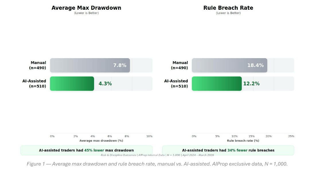
How to read it. Two pairs of horizontal bars. On the left the mean maximum drawdown (axis from 0 to 10 %), on the right the rule-breach rate (axis from 0 to 25 %). One bar in each pair is the manual cohort, the other the AI one.
What to notice. Exactly the same four numbers as in the table above: 7.8 % against 4.3 % and 18.4 % against 12.2 %. The figure adds not one new fact, it is decorative. The bars are roughly proportional to the values, the scale is not truncated, and there is no sleight of hand in the graphics themselves.
The practical takeaway. Note what the figure does not have: confidence intervals. The table has them, and for the breach rate they are 15.1–22.1 % against 9.5–15.4 %. On the figure the two bars look like two exact numbers.
The seven biases and how they are measured
This is the most useful part of the paper. Every behavioural bias is reduced to a rule computed from the trade log automatically.
| Bias | What it is | How it is measured | Weight in the index |
|---|---|---|---|
| Disposition effect | selling profits early, holding losses long | ratio of holding time for losers to winners per session; score = max(0, ratio − 1.0) × 10, capped at 100 | 22 % |
| Loss aversion | moving the stop, holding beyond the allowance | share of trades where the stop was moved away from entry after opening | 20 % |
| Overconfidence | overtrading, oversizing | deviation of trade frequency from a 30-day baseline plus the coefficient of variation of position size | 18 % |
| Anchoring | fixation on the entry price and round numbers | share of trades with a stated target closed by hand at a different level with no record of a changed thesis | 14 % |
| Mental accounting | treating session profit as house money | an increase in position size after session profit above 1.5 daily averages | 12 % |
| Herding | chasing entries | share of entries after a move of 1.5 average daily ranges with no plan | 8 % |
| Recency and revenge | impulsive revenge after a loss | share of entries within 30 minutes of being stopped out, at equal or larger size | 6 % |
The weights are calibrated by logistic regression on the outcome «breach event» over a 2022–2023 training set of 3,400 accounts. The weights sum to exactly 100 %, which checks out.
Three additional metrics:
- Discipline Score, 0–100 is the share of trades that passed all five plan-conformance checks. The mean score is 51.3 by hand against 73.8 with AI.
- The risk adherence index is the share of trades within the stated per-trade risk. 61.4 % against 88.9 %, with a correlation of 0.74 with the account outcome (p < 0.001).
- An emotional exit is any exit where the stop was moved, or the exit was unplanned, or an entry followed within 30 minutes of being stopped out.
Sample composition
| Cohort | N | Share | Account stage |
|---|---|---|---|
| By hand, no AI and no advisors | 490 | 49.0 % | 277 evaluation / 213 funded |
| AI-assisted discretionary | 183 | 18.3 % | 101 / 82 |
| Rule-based expert advisor | 198 | 19.8 % | 112 / 86 |
| Hybrid: AI plus human control | 129 | 12.9 % | 68 / 61 |
| Total | 1,000 | 100 % | 558 / 442, about 128,000 trades |
All the sums recompute and agree: the AI sub-cohorts give 510, the stages give 558 and 442.
3. What does not add up
3.1 One of the seven relative changes is computed wrongly
A recount of all seven headline percentages:
| Metric | From and to | Recount | Claimed |
|---|---|---|---|
| Drawdown | 7.8 → 4.3 | 44.9 % | 45 % ✓ |
| Emotional exits | 61.7 → 37.2 | 39.7 % | 41 % ✗ |
| Sharpe | 0.62 → 0.89 | 43.5 % | 44 % ✓ |
| Breaches | 18.4 → 12.2 | 33.7 % | 34 % ✓ |
| Risk adherence index | 61.4 → 88.9 | 44.8 % | 45 % ✓ |
| Profit factor | 1.21 → 1.58 | 30.6 % | 31 % ✓ |
| Holding time | 4.1 → 1.7 | 58.5 % | 59 % ✓ |
Six of the seven are rounded correctly. The seventh, the reduction in emotional exits, gives 39.7 % while 41 % is claimed. The summary says "Emotionally-driven exits: 37.2% (AI) vs. 61.7% (manual) — 41% reduction", and the conclusions say "AI-assisted trading associated with 41% fewer emotionally-driven exits". The figure is repeated three times: in the abstract, in the summary and in the conclusions section. The error is small in magnitude, but it is the only one in a set where all the others are accurate, and it is biased in the convenient direction.
3.2 The chi-square matches none of the stated sample sizes
The conclusions say, verbatim: "37.2% vs. 61.7% (−24.5 pp; chi-square = 142.3; p < 0.001)".
What a chi-square is. A measure of the discrepancy between observed frequencies and those expected under no association. It grows with sample size: the same difference in percentages gives a large value on a large sample and a small one on a small sample. So from the value of a chi-square one can recover how many observations there were.
A recount under different units of observation:
| Unit of observation | n per group | Chi-square |
|---|---|---|
| Traders | 490 / 510 | 60.0 |
| Trades (about 128,000 split in half) | 64,000 / 64,000 | 7,684 |
| What matches the stated value | ≈ 1,186 / 1,186 | 142.4 |
The stated value of 142.3 matches neither the number of traders nor the number of trades. It matches a sample of about 1,186 observations per group, that is, roughly 2,370 exits in total, and no such quantity appears anywhere in the paper. The denominator of the headline significance test is not named and cannot be recovered from the text.
This is not a trifle: emotional exits are stated as a share of exits, not of traders, and with 128,000 trades there should be two orders of magnitude more exits. Either the test was run on a subsample that is not mentioned, or the value was computed on data other than the data described.
3.3 The same number, 73 %, denotes two different claims
In the table of seven biases, the revenge row, key-statistic column:
"73% of manual breaches had revenge trade as trigger"
In the conclusions section:
"Behavioral failures — not strategy — drive 73% of breaches. In the manual cohort, 73% of breach events (66/90) were preceded by a BBI-tagged behavioral event (loss aversion stop-removal, revenge entry, or mental accounting oversize) in the same session."
These are two different claims. In the first, 73 % is attributed to one bias out of seven. In the second, to the union of three. Both cannot be true. A contradiction check: in the same table, loss aversion is credited with "Drives 34.2% of manual breaches". If revenge accounts for 73 % and loss aversion for 34.2 %, the sum is already 107 % while these are two terms out of three. The ratio 66/90 = 73.3 % confirms that the arithmetic in the conclusions refers to the union, and the table row is the erroneous one.
3.4 The comparison with Odean puts unlike quantities side by side
The paper's first conclusion, verbatim: "Disposition effect 2.7× more severe than academic benchmarks. Manual cohort loser/winner hold ratio of 4.1× (95% CI 3.8–4.4×) vs. Odean (1998) benchmark of ~1.5×." The ratio 4.1/1.5 = 2.73, and the arithmetic is right.
What is wrong is the comparison itself. Odean's measure of disposition is the ratio of the proportion of gains realised to the proportion of losses realised: out of all paper gains, what fraction the trader locked in, and likewise for losses. Here what is measured is the ratio of holding times for losing positions to winning ones. These are different quantities with different units and different distributions, and there is no reason for them to coincide even under identical behaviour. Comparing them and declaring a 2.7-fold difference is a substitution.
A monetary estimate is then derived from it: "For \$50K–\$100K accounts, the implied annual performance cost is \$2,200–\$4,400 (Odean: 4.4% return drag)". That is, Odean's 4.4 % coefficient is taken and applied to account sizes. But if disposition here is 2.7 times stronger than in Odean, the loss should not equal his 4.4 % either. Either the effect is stronger and the loss is larger, or the loss is the same and the effect is not stronger.
3.5 Two of the three AI sub-cohorts are not statistically different from the manual one
| Sub-cohort | Breach rate (95 % CI) | Sharpe | Risk index |
|---|---|---|---|
| By hand (benchmark) | 18.4 % (15.1–22.1) | 0.62 | 61.4 % |
| AI-assisted discretionary | 15.1 % (10.4–21.1) | 0.81 | 79.2 % |
| Rule-based expert advisor | 13.6 % (9.5–18.8) | 0.91 | 91.3 % |
| Hybrid AI and human | 8.5 % (4.8–14.4) | 0.97 | 94.1 % |
The discretionary sub-cohort's interval (10.4–21.1) overlaps the manual one (15.1–22.1) across six points. The rule-based advisor's interval (9.5–18.8) overlaps across three and a half. The difference is not established for either of these two groups. Only the hybrid does not overlap, and even then by seven tenths of a point.
The paper prints this table and says not a word about the overlap. The headline figure of «34 % fewer breaches» is obtained by pooling three sub-cohorts, two of which taken separately are indistinguishable from the benchmark.
3.6 A rule-based advisor is not AI
198 traders out of the 510 in the AI cohort, that is 38.8 %, fall into the category of a deterministic advisor executing written rules. That is automation, not artificial intelligence, and the technologies differ about as much as technologies can. The paper explains the mechanism itself: "Improvement was largest in Rule-Based EA and Hybrid sub-cohorts where execution rules make emotional patterns structurally impossible."
And that is the real conclusion the data supports: the gain comes from removing manual intervention, not from the intelligence of the tool. Labelling the result an achievement of AI is a marketing decision.
3.7 The drawdowns are truncated by the rules themselves
A mean maximum drawdown of 7.8 % and 4.3 % over 24 months is suspiciously small for retail traders. The explanation is simple: on a prop account the drawdown is capped by the firm's rules, usually around 10 %, and on reaching it the account dies. So the observed drawdown distribution is censored from above, and the difference between cohorts is measured not on the full distribution but on what survived.
The inclusion criteria belong here too: an active account, at least 20 completed trades, at least 5 active days. A trader who blew up in three days does not enter the sample. Interestingly, this bias works against the paper's conclusion: it is usually manual traders who blow up faster, and screening them out improves the manual cohort. But the very fact that two different selections act simultaneously in opposite directions means the size of the effect cannot be extracted from this data at all.
3.8 Self-selection, named but not removed
Assignment to cohorts is self-selected: people decided for themselves whether to use AI. The paper acknowledges this in its limitations and correctly writes «associated with» throughout. But the headline figures are nonetheless presented as an effect of the tool, including the recommendation to deploy AI guardrails. A trader who chose an AI tool would in all likelihood have been more disciplined without it too, and the correlation of the risk index with the outcome (0.74) reads just as well as «disciplined people are both disciplined and profitable».
3.9 A number with no source
In the bias table, the overconfidence row, key-statistic column: «affects about 70 % of retail traders». This is a claim about an external population rather than about the paper's sample, and it carries no reference. The bibliography has six entries, and none of them is attached to this number; the last of them is given without an author, journal name or identifier, so it is not a reference in any verifiable sense.
4. What is worth taking from it
Despite everything listed above, one thing in the paper is done well and applies directly: seven behavioural biases are turned into rules computed from the trade log with no need to question the trader. None of them requires knowing what the person felt; all rely on timestamps, prices and sizes.
It is useful in one specific place. A portfolio of systematic strategies does not experience the disposition effect: it has no mechanism for holding a loss longer than a profit. But the person sitting over that portfolio does have one, and it shows up in manual intervention: pulling a stop, closing early, adding size after a good day, restarting a halted strategy after a run of losses. Those interventions leave exactly the traces described here.
Three metrics worth computing on your own log:
The share of trades where the stop was moved after opening. For a fully automatic system this is zero by definition. Any non-zero value is precisely a measure of manual intervention, and it is computed in one line over the log.
The risk adherence index: the share of trades within the stated per-trade risk. For a systematic portfolio this checks that position size matches what was computed. A discrepancy points either to a manual edit or to a defect in the sizing.
The share of entries within 30 minutes of being stopped out, at equal or larger size. For an automaton this is a property of the strategy rather than an emotion, but the metric is useful all the same: it shows how many times the system re-enters straight after a loss, and whether such re-entries are worth restricting.
Worth noting separately is the thesis the paper states as its main one, and which, unlike the percentages, survives a check by logic: prop-firm rules screen out behaviour, not skill. It is the same thought the Youngblood paper arrives at independently from the opposite side, by showing that a fixed position size makes several rules inoperative. Two sources, different methods, one conclusion.
5. Testable ideas
| No. | Idea | Type | Where to compute |
|---|---|---|---|
| 1 | Compute on your own log the share of trades where the stop was moved after opening: for an automatic portfolio the norm is zero, and any deviation measures manual intervention | acceptance metric | Python |
| 2 | Risk adherence index: the share of trades whose actual risk landed in the stated corridor. A discrepancy points to a sizing defect or a manual edit | acceptance metric | backtester |
| 3 | The share of entries within 30 minutes of being stopped out, at equal or larger size; test whether banning such re-entries improves the portfolio's result | design change | backtester |
| 4 | The ratio of median holding time for losing trades to winning ones, per strategy: for symmetric exits about 1 is expected, and a large deviation signals asymmetric exit rules | diagnostic | Python |
| 5 | The coefficient of variation of position size per strategy: with correctly working sizing it is determined by volatility alone, and spikes point to a bug | audit | backtester |
| 6 | Check whether the drawdown distribution is censored by account rules before comparing mean drawdowns between any groups | audit | Python |
| 7 | When comparing subgroups, always look at the overlap of confidence intervals rather than point estimates alone: in this paper two sub-cohorts out of three are indistinguishable from the benchmark | acceptance metric | any |