How to read this walk-through. The paper has two parts of different weight. Its core is the formulas themselves: appendix A, where 101 alphas are written in a small language of operators. Section 2 walks through that language, section 3 goes through several alphas step by step, and section 4 sums up the whole catalog in a table of groups. The second part of the paper, the empirics on proprietary data, is covered in section 5; its numbers cannot be checked. We do not go through all 101 formulas one by one: they are publicly available at the link.
The main thesis
The author publishes 101 trading alphas for US stocks as explicit formulas. From the abstract: "We present explicit formulas – that are also computer code – for 101 real-life quantitative trading alphas." The formulas are short and written in a language of two dozen operators, so once the operators are defined, every formula runs as code.
The alphas belong to WorldQuant LLC and are published with its permission. In the conclusion the author stresses that these are not textbook examples: "In fact, 80 of these alphas are in production as of this writing." Which 80 exactly is not stated: "For proprietary reasons, we are not at liberty to state precisely which ones."
The formulas come with three empirical results on the alphas themselves for 2010–2013:
- the average holding period is roughly 0.6 to 6.4 days, that is, a high- and mid-frequency horizon;
- the average pairwise correlation of the alphas is low: 15.9 %, median 14.3 %;
- an alpha's return grows with its volatility but has no significant dependence on turnover; and turnover explains the correlations between alphas poorly.
These 101 alphas were not picked at random: "We picked these alphas largely based on simplicity considerations", so that they could fit into a paper. The author notes that there are many other, “non-formulaic” alphas that are too complex to publish.
1. What is called an alpha here
The author gives the definition from the WorldQuant book (Tulchinsky et al., 2015): an alpha is a combination of mathematical expressions, code and configuration parameters that, together with historical data, makes it possible to forecast the movement of instruments. And immediately clarifies: here the word is used in the trader's sense, as any reasonable forecast of expected return that can be traded on, and this is not necessarily the same as the “academic” alpha, the residual of a regression on risk factors.
Why so many alphas. In the introduction the author describes two opposing trends. More and more participants search for alphas with quantitative methods, and the alphas themselves become weaker and shorter-lived as a result: "This results in ever fainter and more ephemeral alphas." On the other hand, the search for alphas can largely be automated, and their number runs into the hundreds of thousands and millions. What is traded, though, is not individual alphas but a “mega-alpha” assembled from many. The benefits of such a setup, according to the author: internal crossing of trades (a buy from one alpha cancels a sell from another, which saves substantially on costs) and diversification in case some of the alphas stop working. The difficulty of combining them is named too: there are too many variables and too few observations, "Thus, the alpha sample covariance matrix is badly singular."
Mean reversion and momentum. Very roughly, the author writes, alphas fall into these two types. The simplest mean-reversion alpha, formula (2) of the paper:
What this is. A bet that the overnight gap will partially close.
What each symbol means. (“natural logarithm”): for small changes it turns a price ratio into a return, . The minus in front flips the sign.
Step by step, our example. Yesterday's close is 100, today's open 102. The ratio is 1.02, the logarithm about 0.0198, with the minus . The signal is negative: we sell the stock, expecting part of the gap to come back. The author says this directly:
"The idea (or hope) here is that the stock will mean-revert".Why this matters. The example introduces the notion of delay-0: the alpha's data refer to the same moment at which the alpha is traded. This alpha has to be executed at the open or as close to it as possible. Yesterday's close is adjusted for splits and dividends if the ex-date is today.
The simplest momentum alpha, formula (3):
What this is. If the stock rose intraday yesterday, we buy it today, expecting the move to continue.
Why this matters. The example introduces delay-1: the alpha is traded on the day after the date of the most recent data. The author notes that the same formula executed as close as possible to yesterday's close would be delay-0. Delay-2 is defined the same way, with a two-day lag.
Of the 101 alphas in the appendix, four, according to the author's footnote, are delay-0: numbers 42, 48, 53 and 54. They are meant to be executed at the close of the day for which they are computed, or as close to it as possible.
2. The language of the formulas: operators and data
Appendix A.2 defines the operators from which all the alphas are built. All expressions are case-insensitive: Ts_Rank and ts_rank are the same thing.
| Operator | How to read it | What it does |
|---|---|---|
rank(x) |
cross-sectional rank | the rank of the value among all stocks on that day |
delay(x, d) |
delay | the value of days ago |
delta(x, d) |
change | today's minus days ago |
correlation(x, y, d) |
rolling correlation | the correlation of series and over the last days |
covariance(x, y, d) |
rolling covariance | the same for covariance |
ts_min(x, d), ts_max(x, d) |
minimum, maximum over time | the minimum or maximum of over days |
ts_argmax(x, d), ts_argmin(x, d) |
day of the maximum, minimum | on which of the last days the maximum or minimum occurred |
ts_rank(x, d) |
rank over time | the place of today's among its values over days |
sum(x, d), product(x, d) |
sum, product | over the last days |
stddev(x, d) |
rolling standard deviation | the spread of over days |
decay_linear(x, d) |
linearly decaying average | the average over days with weights , normalized to sum to 1 |
scale(x, a) |
normalization | rescales so that the sum of absolute values across stocks is (1 by default) |
signedpower(x, a) |
power | defined in the paper as |
indneutralize(x, g) |
industry neutralization | subtracts from the mean of its group: sector, industry, subindustry |
x ? y : z |
condition | if is true, then , otherwise |
An important rule for all operators of the form ts_…: "non-integer number of days d is converted to floor(d)", that is, a fractional number of days is rounded down. This is worth knowing because in the second half of the catalog the windows are given by numbers such as 16.1219.
Input data (section A.3): returns (close-to-close return), open, close, high, low, volume, vwap (the day's volume-weighted average price), cap (market capitalization), adv{d} (average daily dollar volume over days, for example adv20) and IndClass, a placeholder for any industry classification: GICS, BICS, NAICS, SIC. The author notes that different IndClass in one alpha do not have to refer to the same classification.
Why
rankis almost everywhere. The definition in the paper is a single phrase:"cross-sectional rank". The meaning is this: what matters is not the size of the signal but the place of the stock among the others on the same day. This dampens outliers (the stock that fell the most gets the highest rank whether it fell by 15 % or by 40 %), makes the signal comparable from day to day at any overall volatility, and automatically makes the strategy cross-sectional: stocks are compared with each other, not each with its own past. How exactly the rank is normalized is not stated in the paper; formulas such asrank(...) - 0.5and0.5 < rank(...)show that a fraction from 0 to 1 is implied. This is our reading.
3. Several alphas step by step
Below are six alphas chosen to show the main devices of the language. The author's explanations exist only for alphas 42 and 101; the other readings are ours.
Alpha#101: the share of the day traveled end to end.
((close - open) / ((high - low) + .001))What this is. How much of the whole daily range the move from open to close covered. The value is about if the day opened at the low and closed at the high, about in the opposite case.
What each symbol means.
close - open: the change over the day.high - low: the daily range..001: an addition that protects against division by zero when the high equals the low.Step by step, our example. Open 100, close 102, high 103, low 99. The numerator is 2, the denominator , the signal about 0.5.
Why this matters. The author calls it a delay-1 momentum alpha:
"if the stock runs up intraday (i.e., close > open and high > low), the next day one takes a long position in the stock".
Alpha#33: reversal of the intraday move, via rank.
rank((-1 * ((1 - (open / close))^1)))What this is. If the close is above the open,
open / closeis less than one, the expression1 - open/closeis positive, and after multiplying by it is negative. The stocks that rose the most over the day get the lowest rank, those that fell the most the highest.What each symbol means.
^1: raising to the first power, changes nothing.rank(...): the place of the stock among all stocks on that day.Step by step, our example. Five stocks with daily changes of +3 %, +1 %, 0 %, −2 %, −5 %. The values inside the rank are roughly −0.03, −0.01, 0, +0.02, +0.05. If the rank is normalized from 0 to 1, this gives 0, 0.25, 0.5, 0.75, 1: we buy the most of the one that fell 5 % and sell the most of the one that rose 3 %.
Why this matters. This is mean reversion on a one-day horizon. It is not on the delay-0 list, so it is traded on the day after the calculation.
Alpha#42: where the price closed relative to vwap.
(rank((vwap - close)) / rank((vwap + close)))What this is. According to the author, essentially a delay-0 mean-reversion alpha. If the close is above
vwap, the stock rose in the second half of the day, the numerator is small, and the rank is low. The denominator, as the author writes,"weights down richer stocks", that is, it reduces the weight of expensive stocks.Why this matters. The position “against the move” is opened close to the close of the same day. This is one of the four alphas for which execution at the moment of calculation is mandatory.
Alpha#12: a price change whose sign is set by volume.
(sign(delta(volume, 1)) * (-1 * delta(close, 1)))What this is, our reading.
delta(close, 1): the change in the closing price over the day.sign(delta(volume, 1)): if volume rose compared with yesterday, if it fell. When volume rises, the alpha bets against yesterday's price move; when it falls, with the move.Why this matters. An example of how one field (volume) switches the direction of the bet on another (price).
Alpha#6: rolling correlation of price and volume.
(-1 * correlation(open, volume, 10))What this is, our reading. The correlation of the opening price and volume over the last 10 days, with the opposite sign. A stock whose price rise came on rising volume gets a negative signal.
Why this matters. Rolling correlations between price and volume appear in 60 alphas out of 101 (our count); this is the most frequent operation after rank.
Alpha#9: a streak versus a single move.
((0 < ts_min(delta(close, 1), 5)) ? delta(close, 1) : ((ts_max(delta(close, 1), 5) < 0) ? delta(close, 1) : (-1 * delta(close, 1))))What this is, our reading. If all daily price changes over the last 5 days are positive (their minimum is above zero), the alpha goes with today's change. If all are negative (the maximum is below zero), also with it. In all other cases against it.
Why this matters. Momentum and mean reversion are mixed within a single formula: after a steady streak the alpha follows the market, after days going in different directions it bets on a pullback. The author writes that in complex alphas these elements get mixed and the alphas themselves become less definite in type.
What the second half of the catalog looks like. Starting from number 58, the formulas are built differently:
Alpha#61: (rank((vwap - ts_min(vwap, 16.1219))) < rank(correlation(vwap, adv180, 17.9282)))Windows such as 16.1219 and 17.9282 days are rounded down to 16 and 17 by the paper's rule. There are also mixes of a field with itself, for example ((vwap * 0.728317) + (vwap * (1 - 0.728317))), which equals simply vwap. In appearance this looks like the output of machine parameter fitting, but the paper says nothing about it; this is our assumption.
4. What the 101 alphas are made of
A summary of appendix A. The count is ours, from the text of the formulas; one alpha can fall into several rows.
| Feature | Alphas | Numbers or example |
|---|---|---|
Cross-sectional rank rank |
77 | for example 1, 33, 42 |
Volume (volume or adv{d}) |
70 | for example 3, 6, 12 |
| Rolling correlation or covariance | 60 | for example 2, 3, 6, 13 |
Volume-weighted average price vwap |
43 | for example 5, 42, 57 |
Rank over time ts_rank |
38 | for example 4, 7, 17 |
| Fractional windows such as 16.1219 | 40 | 58–99, except 60 and 83 |
Linearly decaying average decay_linear |
22 | for example 31, 39, 57 |
Industry neutralization indneutralize |
18 | 48, 58, 59, 63, 67, 69, 70, 76, 79, 80, 82, 87, 89, 90, 91, 93, 97, 100 |
| Only the day's prices, without volume, vwap, returns or industries | 16 | 4, 9, 10, 18, 20, 23, 24, 33, 37, 38, 46, 49, 51, 53, 54, 101 |
Condition ? : |
11 | 1, 7, 9, 10, 21, 23, 24, 27, 46, 49, 51 |
| Windows from 200 to 250 days | 7 | 19, 32, 36, 37, 39, 48, 52 |
| Delay-0, per the author's footnote | 4 | 42, 48, 53, 54 |
Market capitalization cap |
1 | 56 |
The author describes the catalog this way: these are mostly “price–volume” alphas, and “fundamental” data are used in some: market capitalization in one, and industry classification for neutralization in a number of alphas.
5. Empirical properties of the alphas
How they were measured
The data are proprietary, from WorldQuant, for the period from January 4, 2010 to December 31, 2013. "The number of observations in the time series is 1,006". For each alpha:
What this is. Three metrics of alpha number : the annual Sharpe, the daily turnover, and the profit in cents per share traded.
What each symbol means.
- : the average daily P&L in dollars. : the daily volatility of the portfolio in dollars. (“the square root of 252”): converts the daily Sharpe into an annual one, 252 trading days a year.
- : the average daily turnover in dollars. : the total investment in the alpha, long plus short positions, without leverage. = 0.5 means that half of the portfolio is retraded in a day; is the average holding period in days.
- : the average number of shares traded per day (buys plus sells). The factor 100 converts dollars into cents.
A worked example on the paper's numbers. The highest turnover in table 1 is 1.604 per day, the shortest holding period 0.6235 days. The lowest turnover is 0.1571, the longest holding period 6.365 days. Hence the range “0.6–6.4 days” in the abstract.
Why this matters. Cents per share are directly comparable with costs: if commission, half the spread and price impact together exceed cents per share, the alpha loses money after costs. This is our conclusion from the definition; it is not in the paper.
Next, from the sample covariance matrix of the alpha returns, the daily volatility and the correlations are taken, as well as the average daily return and the annual one . On these data the matrix is nonsingular: 101 alphas on 1,006 observations.
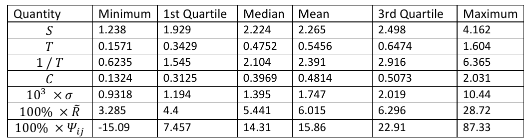
How to read it. Rows: the annual Sharpe , the daily turnover , the holding period , cents per share , the daily volatility (multiplied by 1,000), the annual return in percent, the pairwise correlations in percent. Columns: minimum, first quartile, median, mean, third quartile, maximum.
What to notice. The median Sharpe is 2.224 with a minimum of 1.238: there are no weak alphas in the catalog. The median annual return is 5.441 % with a median daily volatility of 1.395 thousandths, that is, about 0.14 % a day. The median of cents per share is 0.3969, that is, roughly 0.4 cents of profit on each share traded before costs. Correlations range from −15.09 % to 87.33 % with a mean of 15.86 %.
The caveat under the table.
"The performance figures are exclusive of any trading or transaction costs, price impact, etc."
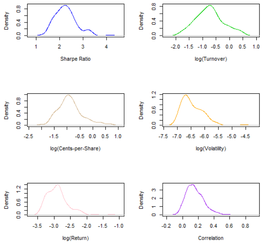
How to read it. Each panel shows how one metric is distributed across the 101 alphas (across the pairwise correlations for the last panel). Turnover, cents, volatility and return are given in logarithms.
What to notice. Turnover is distributed roughly lognormally, which is why its logarithm is used in the regressions that follow. The isolated outliers on the right for the Sharpe, volatility and return, according to the figure caption, come from the delay-0 alphas. The correlations are concentrated around 0.1–0.2.
Return grows with volatility
The author confirms the relationship found earlier on 4,000 alphas (Kakushadze and Tulchinsky, 2015), formula (1) of the paper:
The regression across the 101 alphas with an intercept (table 2):
What this is. The relationship between an alpha's average daily return and its daily volatility, both in logarithms.
What each symbol means. : the natural logarithm. If both sides are in logarithms, the slope of the line becomes the exponent: . The symbol reads “is proportional to”.
Step by step, our example. An alpha has twice the volatility. Then its return is higher by a factor of , not 2, and its Sharpe is about of the Sharpe of the calmer alpha.
A worked example on the paper's numbers. The slope is 0.761 with a standard error of 0.046, the t-statistic 16.65, = 0.737 (adjusted 0.734).
Why this matters. An exponent below one means that more volatile alphas have a lower Sharpe on average: return grows more slowly than risk.
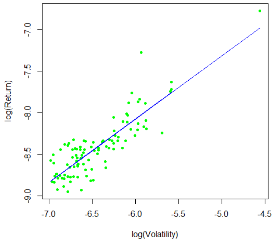
How to read it. Each point is one alpha: horizontally, the logarithm of the daily volatility; vertically, the logarithm of the average daily return. The line is the regression from table 2.
What to notice. The main cloud lies along the line; one point at the top right stands far from the others in volatility. According to the caption of figure 1, the extreme values of volatility and return come from the delay-0 alphas.
Turnover does not explain return
The second regression adds the logarithm of turnover (table 3):
What this is. The same relationship, but with turnover as a second explanatory variable.
A worked example on the paper's numbers. The turnover coefficient is −0.023 with a standard error of 0.040, the t-statistic −0.57: it does not differ from zero. rose from 0.737 to 0.738, the adjusted one fell from 0.734 to 0.732.
Why this matters. This is the claim of the abstract: returns
"have no significant dependence on turnover". The author writes that this is a direct confirmation of an earlier result obtained indirectly: there the volatility was estimated through the Sharpe, cents per share and turnover, while here realized volatility is used.
Turnover hardly explains correlations
The author draws a parallel: an alpha's turnover is like a stock's liquidity, and the logarithm of liquidity serves as a style factor in multifactor risk models. The question: does the logarithm of turnover explain the pairwise correlations of the alphas? The factor model of covariance, formula (7):
What this is. The standard way to write a factor model: the covariance of two alphas is the sum of their own risk and common factors.
What each symbol means.
- (“gamma”): the modeled covariance of alphas and .
- (“xi squared”): the specific, own risk of alpha . (“Kronecker delta”): one when , zero otherwise; the specific risk sits only on the diagonal.
- (“omega”): the loading of alpha on factor . (“phi”): the covariance of the factors. : the number of factors, much smaller than the number of alphas .
Why this matters. The author takes the logarithm of turnover as one of the columns of loadings and checks whether it explains the correlations.
Technically, this is a regression of all pairwise correlations (with 101 alphas that is 5,050 pairs, our calculation) on two quantities built from normalized logarithms of turnover: the sum and the product (table 4):
What this is. An attempt to predict the correlation of a pair of alphas from their turnovers.
What each symbol means. (“psi”): the correlation of alphas and . (“tau”): turnover normalized so that the mean of its logarithm across the alphas is zero.
A worked example on the paper's numbers. The coefficients are formally significant (t = 2.907 and 7.537), but = 0.0127. The intercept of 0.1587 simply reproduces the average correlation.
Why this matters. The author's conclusion: turnover by itself says almost nothing about how similar two alphas are. And a caveat: this
"does not necessarily mean the turnover adds no value in the factor model context". Turnover may help through specific risk, but checking that requires proprietary methods and was not included in the paper.
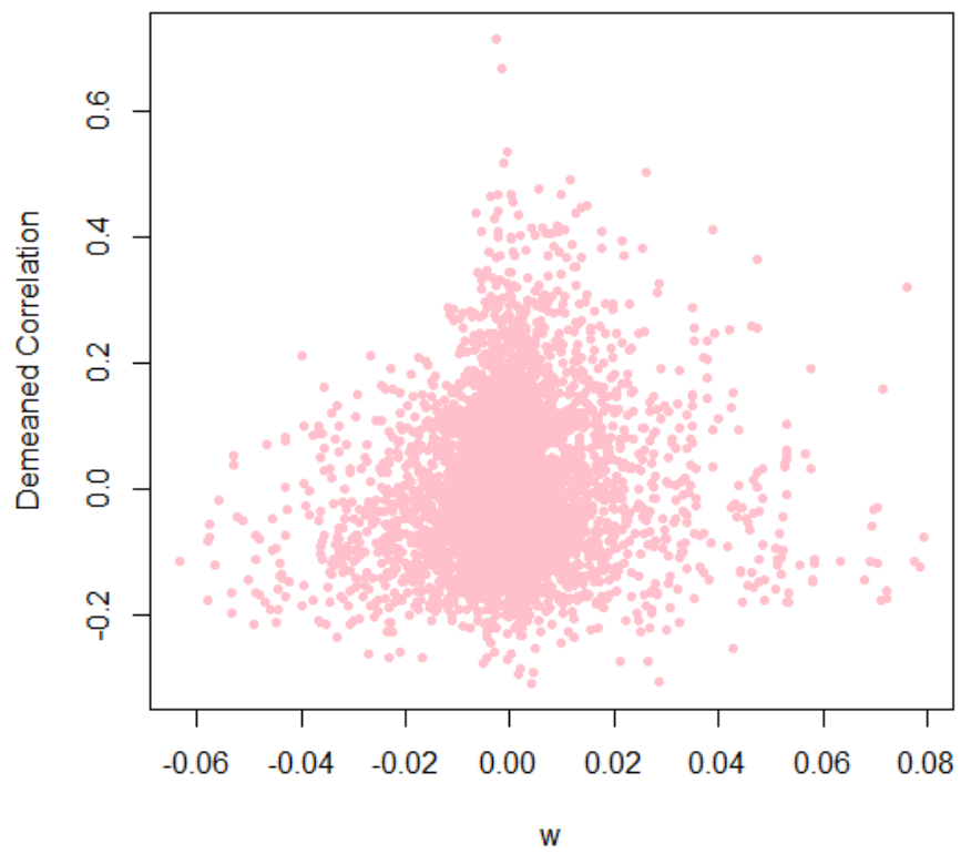
How to read it. Each point is one pair of alphas. Horizontally, the prediction from turnover from table 4; vertically, the deviation of the actual correlation from the mean.
What to notice. The cloud has no slope: if turnover explained the correlations, it would be stretched along the diagonal.
There is, however, a relationship between turnover and volatility, though not a strong one (table 5): , the t-statistic of the slope 5.412, = 0.228.
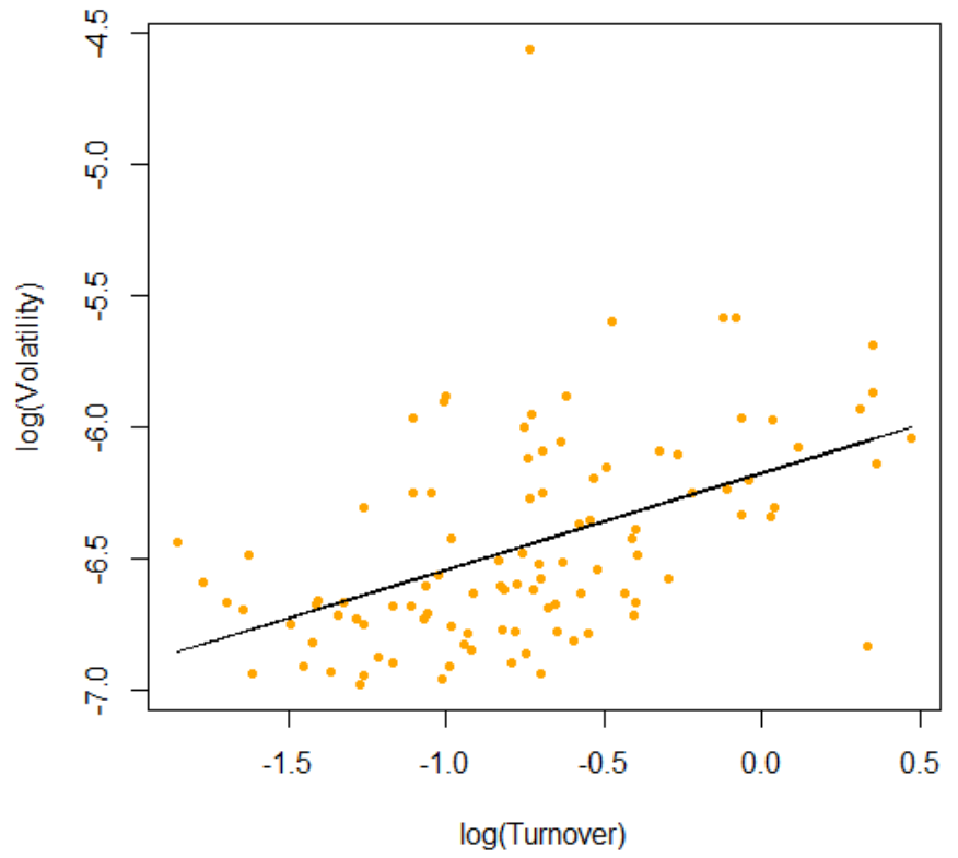
How to read it. Horizontally, the logarithm of turnover; vertically, the logarithm of volatility.
What to notice. Faster alphas are on average slightly more volatile, but the spread around the line is large. In a footnote the author adds that suppressing alpha weights by turnover can add value but is strongly correlated with suppression by volatility.
6. What is shaky in the paper
The author's own caveats
No costs. Under table 1 it says directly that the figures do not include trading costs, price impact and the rest. With a holding period of 0.6 to 6.4 days and a median profit of about 0.4 cents per share, this is the decisive caveat: the Sharpe of 2.2 in the table is a Sharpe before costs.
Selected for simplicity, not at random. The alphas were chosen "largely based on simplicity considerations". This is not a random sample from production, and it is unknown which 80 of the 101 were traded.
Proprietary data. Both the alphas and the data belong to WorldQuant. The author writes that the paper gives as many details as the proprietary nature of the dataset allows. The Sharpes, turnovers and correlations cannot be reproduced; one can only compute the same formulas on one's own data.
Turnover and the risk model. The negative result on correlations does not mean that turnover is useless in a factor model; the author did not test a contribution through specific risk.
What is visible on reading but not discussed in the paper
Our working review has no discrepancies confirmed by a quotation, so discrepancies is zero. We did not recompute the numbers. Below are points that matter for anyone who will rewrite the formulas as code; these are our observations, not errors found.
Two-argument min and max. In the appendix, min(x, d) and max(x, d) are defined only as synonyms for ts_min and ts_max, where the second argument is a number of days. But in nine alphas (71, 73, 76, 77, 82, 87, 88, 92, 96, our count) the second argument is a whole expression, not a number. This can be read in two ways: as the element-wise maximum of two series, or literally as a window equal to the value of the expression. The paper does not say which is meant.
signedpower. Defined as . The name suggests “a power that preserves the sign”, that is, , but the definition does not say so. In alpha 84 the exponent is itself a series.
The rank is not defined in detail. Normalization and the handling of ties and missing values are not described.
The period. Four years, 2010–2013. From this one stretch alone it is impossible to judge how stable the characteristics of the alphas are over time.
How to combine them is not stated. By the paper's own logic, the value is created by the “mega-alpha”, but the paper gives no method of combination.
7. What follows in practice
This is a ready-made specification of a small language for describing alphas. Two dozen operators and about ten input fields cover the whole catalog. If you are building an engine that computes signals from formulas, the 101 alphas serve as a test suite: either the engine computes all of them without manual edits or it does not.
Resolve the ambiguous points in advance and write the decisions down. Two-argument min and max, signedpower, the rounding of fractional windows, the normalization of rank. Different readings give different alphas with the same number.
A single alpha from the catalog is not a strategy. Holding periods are measured in days, and the median profit is about 0.4 cents per share before costs. The author describes the working setup as a combination of many weak signals with internal crossing of trades. Trading one formula on its own with retail costs means taking the wrong part of the system.
Compute cents per share before the Sharpe. It is a direct comparison with the execution cost per share; a Sharpe before costs does not allow such a comparison.
Do not infer the similarity of strategies from their turnover. According to this paper, turnover hardly explains correlations; similarity has to be measured on the returns themselves.
A delay label for every strategy. Delay-0 and delay-1 are different strategies with different execution requirements. A delay-0 alpha executed an hour after the calculation is no longer the same alpha.
8. Testable ideas
| No. | Idea | Type | Where to compute |
|---|---|---|---|
| 1 | Implement all the operators of the appendix and run all 101 formulas as a test suite for the signal engine: each one is computed without manual edits | audit | Python |
| 2 | Fix and document the reading of the ambiguous points: two-argument min/max in nine alphas, signedpower, rounding of fractional windows, normalization and ties in rank |
audit | Python |
| 3 | Compute the pairwise correlations of the returns of your own signals and compare them with the mean of 15.9 % and the median of 14.3 % from the paper: much higher means many variants of one idea | diagnostic | Python |
| 4 | Regress the logarithm of the average return on the logarithm of volatility across your own set of strategies; compare the slope with 0.76 | diagnostic | Python |
| 5 | Check on your own set whether the logarithm of turnover explains return and pairwise correlations; look for a significant turnover effect in the cost model first | diagnostic | Python |
| 6 | For each strategy, record the delay (delay-0, delay-1, delay-2) and verify that the backtester executes trades at exactly that moment | audit | backtester |
| 7 | For several alphas from the catalog, compute the cents per share on your own data and compare with the full execution cost per share | acceptance metric | backtester |
| 8 | Compare combining a group of alphas equally, inversely to volatility and with correlations taken into account: the paper claims the value is in the combination but gives no method | design change | Python |
| 9 | Compare a signal as a cross-sectional rank and as a raw value on the same alpha: the tails of positions and robustness to outliers | design change | Python |