How to read this walk-through. The paper's main idea is explained on one example of ten returns, with no theory: it is in the section “The method in one line”. The formulas below are taken apart symbol by symbol and on numbers; we do not retell the proofs of the theorems, they are in the paper and in the authors' separate articles. If you need only the practical part, read sections 2, 4, 7 and 8. Everything the authors assume and did not check is collected in the section “What is shaky in the paper”.
1. How the problem is set up
There are intraday returns, say five-minute ones, and we need to know how volatile the day was. The standard answer is realized variance: add up the squares of all returns over the day. The theory has long been known: as sampling becomes more frequent, this sum converges to the price's quadratic variation over the day.
What each symbol means. (“y j i”): the -th intraday return of day (a difference of log prices). (“em”): how many observations there are in a day; for the authors is five-minute intervals around the clock. The curly braces with the index are just notation for “sum of second powers”.
Step by step. Square each five-minute return and add them all up.
The problem is that quadratic variation consists of two parts of different nature. If the price moves continuously with its instantaneous volatility and in addition occasionally jumps (news, an unexpected statistic), then
What this is. The day's quadratic variation equals the integrated variance of the continuous part plus the sum of squares of the jumps that occurred during the day.
What each symbol means. (“sigma of u”): instantaneous volatility at time , unobserved. : integrated variance, how much variance the continuous part accumulated over the day. : the size of the -th jump. : the length of the period; for the authors it is a day.
Why this matters. Realized variance sees only the sum. The authors stress:
"realized variance cannot be informative about the separate contributions the diffusion or jump parts of m* make to QV"(section 1.1). To separate them you need either a rigid parametric model or a different statistic. The paper takes the second route.
Why separating is worthwhile can be seen in the market: a day when the price stood calmly except for one five-minute interval after unexpected news, and a day when the price swung widely all day, give similar realized variance. For risk assessment and forecasting these days are different.
2. The method in one line
Instead of the sum of squares, add up the products of absolute values of adjacent returns and multiply by . The result is an estimate of the variance without jumps; the difference with realized variance gives the contribution of jumps.
What this is. Bipower variation in the main special case (both powers equal to one), with a correction factor. In the paper the factor is written as , where , so .
What each symbol means. : the absolute value of the -th return, without its sign. : the absolute value of the next one. The sum runs to because there is one fewer pair of neighbors than returns. The arrow with the letter reads “converges in probability”: as sampling becomes more frequent, the left side comes arbitrarily close to the right side.
Why the jump fades out. A jump falls into one return. In the sum of squares it gets squared. In the sum of products it is multiplied by the neighboring return, an ordinary and small one, and as sampling becomes more frequent the neighbors get ever smaller. In the limit the contribution of rare jumps goes to zero, while the continuous part remains.
A worked example (our example; it is not in the paper). A day of ten returns: nine of 0.1 %, one in the middle of the day of 3 %.
- Realized variance: . The jump gives 99 % of the sum, the day's volatility is .
- There are nine pairs of neighbors. In seven both returns are ordinary: . Two involve the jump: . The sum is .
- Multiply by : , a daily volatility of about 1.03 %.
- The difference : the estimate of the jump's contribution. The true squared jump is ; the shortfall is because with ten observations the jump still noticeably “leaks” into the products with its neighbors. As sampling becomes more frequent, this leakage shrinks.
What this is. An estimate of the jump contribution to the day's variation: realized variance minus bipower variation.
Why this matters. The authors state the paper's contribution this way:
"This seems to be the first method that can separate quadratic variation into its continuous and jump components."(abstract). The conclusions are more cautious:"To our knowledge this is the first radical alternative to the commonly used realized variance estimator of this quantity."(section 6).
3. Formally: power and bipower variation
The paper starts by generalizing realized variance to an arbitrary power, realized power variation:
What this is. The sum of absolute returns raised to the power , with a normalization.
What each symbol means. : the exponent. With we get realized variance, with the sum of absolute values (“realized absolute variation”). : normalization for the sampling frequency. With the exponent is zero and the factor disappears, with it goes to zero as sampling becomes more frequent, with to infinity.
A worked example (our calculation from the paper's formula). day, , : the factor is . The sum of absolute five-minute returns has to be multiplied by 0.059 so that it does not grow just because there are more observations.
The main innovation, realized bipower variation:
What is new. Each term has two adjacent absolute values, each with its own power: (“ar”) on the current return, (“es”) on the next one. The word bipower means exactly “two powers”. With this is power variation again.
The main case . The normalization exponent is , the factor disappears, and what remains is the sum of products of adjacent absolute values, formula (3) of the paper. This is the one line that is implemented in practice.
What converges to what is set by the correction numbers :
What this is. The mean of the absolute value of a standard normal variable raised to the power .
What each symbol means. : the mean (expected value). : the variable is normally distributed with mean 0 and standard deviation 1. (“gamma”): the gamma function, a generalization of the factorial.
Key numbers. : the mean absolute value of a normal variable is smaller than its standard deviation, so the sum of products of absolute values has to be divided by , that is, multiplied by . , so realized variance needs no correction.
Why this matters. Without the correction bipower variation would systematically understate the variance by about a third (, our calculation).
The robustness boundary. Theorem 4 for power variation: with the limit does not depend on rare jumps, with both parts enter, with the limit is determined by the jumps and is infinite. Theorem 5 carries this over to bipower variation: the limit is unchanged by jumps as long as "the maximum of the powers is less than two" (introduction). The authors directly call this the paper's main contribution. With the maximum exactly 2 the limit mixes jumps and volatility; with a larger one it goes to infinity.
In plain terms. A power below two does not let a large value dominate, and the normalization, as sampling becomes more frequent, “damps” a finite number of large terms. The square, by contrast, is built so that a jump's contribution to the sum of squares does not depend on the sampling frequency, and it stays in the limit.
It matters under what assumptions this is proved. The price must be a stochastic volatility process (an integral with respect to Brownian motion) plus a finite number of jumps on any time interval. For theorems 1 and 4 it is additionally required that volatility and drift be independent of the price's Brownian motion, that is, that there be no leverage effect. The general result for bipower variation (section 1.4) the authors state as expected and postpone the proof: "We will discuss a proof of this general result elsewhere.". The special case without drift is proved (theorem 2); after the first version of the article, according to the authors, the condition on the drift was relaxed in a separate paper. On the other hand, the assumptions about jumps are mild: theorem 4 holds for any jump process with a finite number of jumps on an interval, and jumps may depend on each other and on volatility (section 2.2).
4. A check on simulations
The simulation model (section 3.1): variance follows a square-root process (the Heston model) with an average daily variance with and , that is, 0.5 (our calculation from the paper's parameters), , zero drift, no leverage effect by construction. Ten jumps are scattered at random over 50 days, each normal with a variance equal to the variance of 64 % of an ordinary trading day. The authors call them "large but quite rare jumps". The sampling frequencies are , and , that is, every 2 hours, 20 minutes and 5 minutes.
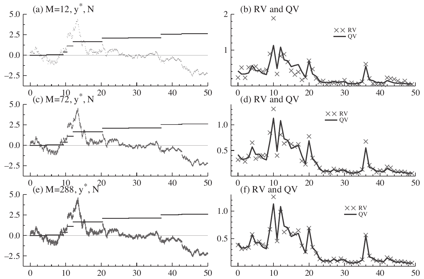
How to read it. The rows correspond to , and . On the left, the price path (as dots, so that the gaps are visible) and a step line that rises at each jump. On the right, crosses: realized variance by day; the line: the true quadratic variation (integrated variance plus squared jumps).
What to notice. As grows, the crosses lie closer to the line. But even at the scatter is noticeable: the authors write that realized variance
"is quite an inaccurate estimator"(section 3.1), although it becomes more precise as grows.
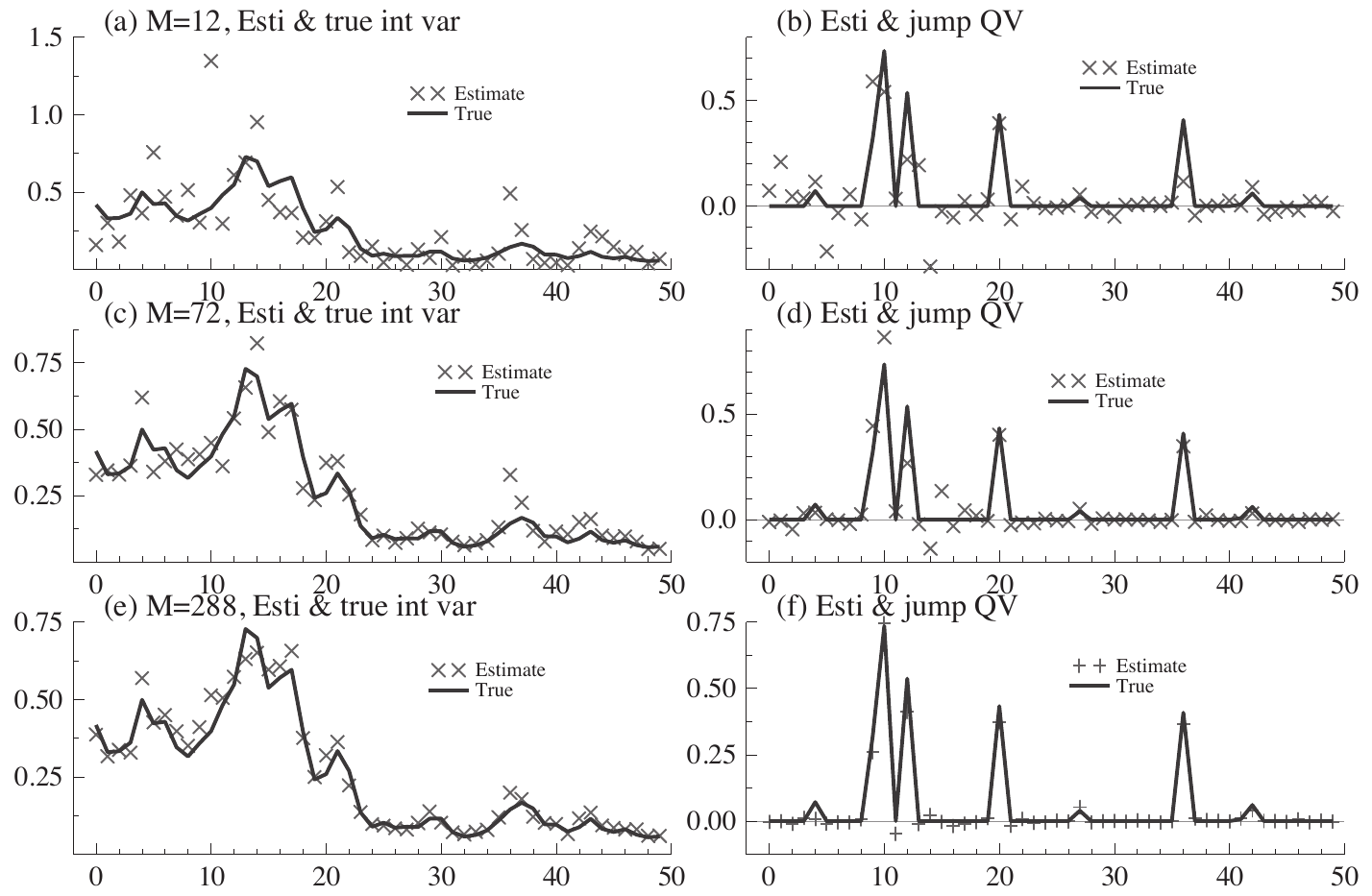
How to read it. On the left, crosses: the estimate of integrated variance ; the line: the true integrated variance without jumps. On the right: the estimate of the jump contribution (realized variance minus bipower variation) against the true one.
What to notice. At on the left there is a cross around 1.35 on the tenth day: the estimate was spoiled by a large jump whose neighbors are not small with two-hour sampling. On the right at there are many negative jump estimates. At and especially the peaks on the right coincide with the real jumps. In the authors' words, for small the jump estimate is
"very inaccurate, but for moderate and large M the estimator works rather well"(section 3.1).
The authors then repeat the experiment on 5,000 days with a jump on average once every 20 days and look at the distribution of errors (table 1). None of the estimates shows much bias. At , 95 % of the errors of realized variance lie between −0.056 and 0.059, of the bipower variation estimate between −0.066 and 0.064, of the jump contribution estimate between −0.033 and 0.037. At the same intervals are −0.294 to 0.262, −0.338 to 0.299 and −0.179 to 0.168. The authors note: "Interestingly, the 95% interval is larger for this error than for the corresponding RV case." (section 3.1). That is, bipower variation estimates its target slightly less precisely than realized variance estimates its own.
Without jumps (table 2) realized variance is also slightly more precise: at the interval is −0.055 to 0.056 against −0.061 to 0.064. The authors: the results "indicate the RV is slightly preferable in terms of accuracy" (section 3.2). This is the price of robustness.
Negative jump estimates. A sum of squared jumps cannot be below zero, but the difference of two estimates can. The authors propose truncating it from below at zero:
What this is. An estimate of the jump contribution that is never negative. Accordingly, the continuous part is estimated as the smaller of two numbers: realized variance and bipower variation.
Step by step. Compute the difference. If it is negative, write zero.
What this gives in table 3 of the paper. At the error shifts to −0.003 on average, but its right tail shrinks to 0.008 against 0.037 without truncation. In other words, the truncated estimate rarely exaggerates jumps much. The price is named by the authors:
"Of course, this estimator has the disadvantage of being biased."(section 3.3).
5. Empirics: the Deutsche Mark/US dollar rate
Data: a five-minute series of the US dollar/German Mark exchange rate from Olsen and Associates, built from bid and ask quotes on the Reuters screen, from December 1, 1986 to November 30, 1996, weekends excluded. All calculations at .
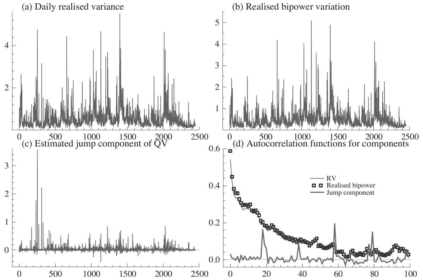
How to read it. (a) Realized variance by day, about 2,500 days. (b) Bipower variation on the same days. (c) Their difference, the estimate of the jump contribution. (d) The autocorrelation of the three series at lags up to 100 days: thin line realized variance, squares bipower variation, thick line the jump contribution.
What to notice. Series (a) and (b) are similar: according to the authors, the estimate of integrated variance makes up the bulk of realized variance. The jump series (c) is mostly around zero with rare outliers, especially at the start of the sample, and there are negative values. Its autocorrelation (d) is around zero: jumps depend weakly on past jumps. The autocorrelation of bipower variation is slightly higher than that of realized variance.
The practical takeaway. If the persistence of volatility matters for a forecast, the jump-cleaned series holds persistence slightly better. The authors call this increase
"quite modest". The paper has no forecasts based on these series; the authors refer to the later work by Andersen, Bollerslev and Diebold (2003), where such models were built.
The average jump contribution to daily quadratic variation is 0.0310 with an average realized variance of 0.528. The authors conclude that "the size of the jump component is quite modest for the dataset" (section 4); as a share this is about 6 % (our calculation).
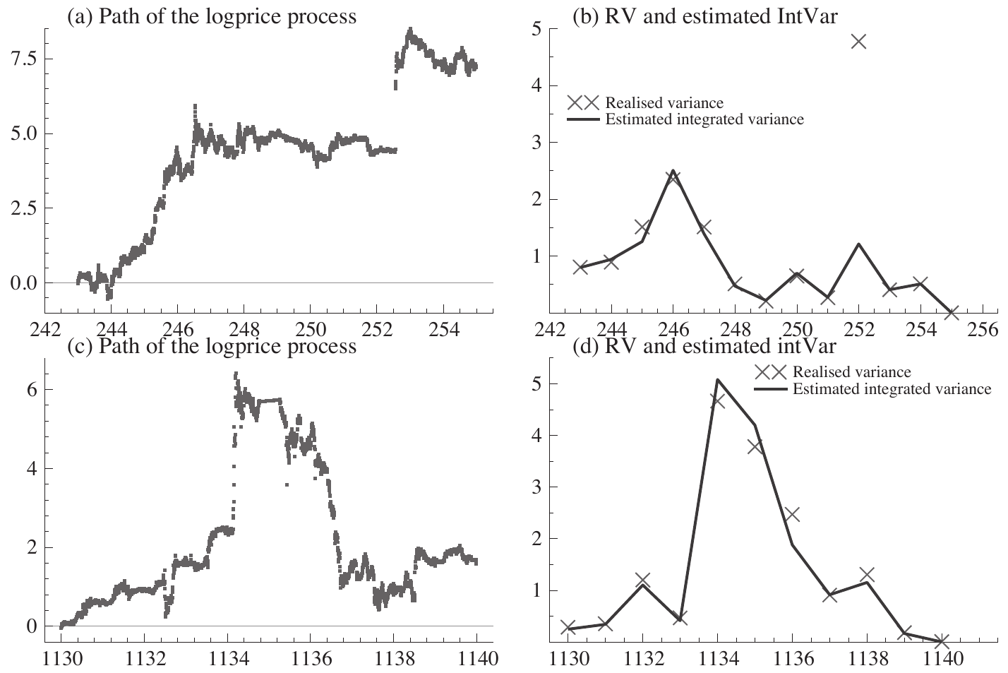
How to read it. The top row: January 15, 1988, when an unexpected US trade balance figure came out. On the left, the price at five-minute intervals as dots; on the right, by day, crosses of realized variance and a line of the integrated variance estimate. The bottom row: August 19, 1991, the day of the coup against Gorbachev.
What to notice. In 1988 the price jumped almost 2 % within one five-minute interval. Realized variance that day is about 4.8, the estimate of integrated variance about 1.2: the statistic attributed most of the day to the jump. In 1991 the price rose by three log units in an hour through a series of positive returns. Realized variance and the estimate of integrated variance are both high, and the authors write:
"the statistics have not flagged up a jump in the price, even though prices were moving rapidly in one direction"(section 4).The practical takeaway. The method finds an isolated gap but does not find a fast move stretched over many adjacent observations: there, every large return has large neighbors too. For a market where news-driven moves come as a cascade over several minutes, this is a significant limit of the method.
6. Extensions
Robust covariance. Via the identity the covariance of two prices can be obtained from three variances: of the sum, of the first price and of the second. If each is estimated through bipower variation, the covariance also becomes robust to jumps (section 5.1). The authors promise to treat this separately.
Multipower variation. More neighbors can be multiplied. Tripower variation with exponents 2/3 and quadpower variation with exponents 1/2 also estimate integrated variance (figures 6–8 of the paper); according to the authors, the answers are not very different. For quadpower variation the jump estimate in one period is strongly negative, and truncation at zero helps again.
Infinitely many small jumps. For Lévy processes with an infinite number of jumps on an interval (the normal gamma process, the normal inverse Gaussian process) the question remains open: "Here we explore this problem, without giving a complete solution." (section 5.3). The authors believe the results carry over to the finite variation case and refer to the later work by Woerner (2003).
The jump test. This is the most practical part of section 5. From the joint limiting distribution of the two estimates (derived in a separate paper by the authors) it follows that without jumps their difference, normalized by the square root of integrated quarticity, is asymptotically normal with variance 0.6091. The asymptotic correlation of the two estimates is about 0.875, and "there is relatively little additional information in the realized bipower variation compared to the realized variance" (section 5.4): the optimal combination of the two estimates without jumps gives realized variance a weight of about one and bipower variation about zero.
The authors recommend the logarithmic form of the test (formula 26 of the paper). In single-day notation, where the ratio of the sampling interval to the period length is :
What this is. The statistic for the test “there were no jumps on this day”. If there are no jumps, is approximately a standard normal variable; if there were, realized variance is noticeably larger than bipower variation, and is large and positive.
What each symbol means. RV: the day's realized variance. BP: the sum of products of adjacent absolute values; BPV: the same with the factor . QPV: the sum of products of four adjacent absolute values. The numerator is the difference of the logarithms of RV and BPV. In the denominator, 0.6091 is the asymptotic variance of the difference, a constant from the paper. The ratio with four adjacent absolute values estimates how unevenly volatility was distributed within the day; the keeps this estimate from falling below , the value for constant volatility.
Step by step. Compute the sum of squares and the sum of products of adjacent absolute values with the factor , take logarithms, subtract. Compute the sum of products of four adjacent absolute values, divide by the square of the sum of products of two adjacent ones, compare with and take the larger. Multiply by 0.6091, take the square root, divide the difference by it. Compare with the one-sided critical value: 1.64 for the 5 % level, 2.32 for 1 %.
What the authors got (table 4). On the Deutsche Mark/US dollar rate the “no jumps” hypothesis is rejected on 21.5 % of days at the 5 % level, on 11.9 % at the 1 % level, on 6.0 % at the 0.1 % level and on 3.83 % at the 0.01 % level.
Why this matters. A daily “there was a jump today” flag with a clear significance level. The authors refer to independent simulations by other researchers in which the transformed (logarithmic) versions of the test
"are reasonably well behaved in empirically reasonable sample sizes"(section 5.4).
7. What is shaky in the paper
The authors' own caveats
Robustness is partial and in places only theoretical. In the abstract both variations are called "somewhat robust to rare jumps", and the separation of risks works "in theory" (section 2.3). The general theorem for bipower variation is stated as expected; special cases are proved.
The independence assumption is not verified. About the requirement that volatility and drift not depend on the price's Brownian motion, the authors write: "It is thus far unclear to us how substantial is the impact of relaxing the independence condition" (section 1.3). In the simulation the leverage effect is excluded by construction: "We rule out leverage" (section 3.1). In the stock market, where volatility rises as the price falls, this assumption is clearly violated; how much this spoils the estimate, the paper does not say.
The number of jumps is finite. For processes with an infinite number of small jumps there is no solution (section 5.3).
Without jumps there is a loss of precision. Table 2 and the asymptotics of section 5.4 show that bipower variation is slightly worse than realized variance when there are no jumps.
The jump estimate can be negative, and truncation introduces bias. Section 3.3.
A series of large returns in a row is not recognized as a jump. The day of the coup, August 19, 1991 (section 4 and figure 5).
What a reading shows
Microstructure noise is not discussed in the paper. The word noise does not occur in the text of the article. All results are asymptotic in the sampling frequency, but on real data with too frequent sampling the price bounces between bid and ask, and both estimates get inflated. The Olsen data themselves are built from bid and ask quotes and preprocessed (with a reference to an appendix of another paper by the authors). The authors call the choice typical for such methods but do not justify it with respect to noise. This is our remark.
Empirics on one series. One exchange rate, one period 1986–1996, one sampling step. Transfer to stocks, futures or cryptocurrencies with their overnight gaps, sessions and liquidation cascades is not tested in the paper.
21.5 % of days with a jump at the 5 % level is hard to interpret without a check of the test's size. This is noticeably more than 5 %, but how well the test holds its nominal level in finite samples is not shown in this paper; the authors refer to simulations by others. This is our remark.
8. What follows in practice
There is one line of code for a variance insensitive to isolated gaps. over intraday returns. Where volatility is used for position size, a single outlier candle stops inflating the estimate and cutting the position the next day.
A separate “jumps of the day” series appears. The difference between realized variance and bipower variation, truncated at zero. According to the paper this series is almost not autocorrelated, that is, jumps are poorly predicted by past jumps, unlike volatility itself.
Frequent data are needed. In the simulation with two-hour sampling the jump estimate is very imprecise; with 20-minute and 5-minute sampling it works. On daily bars the method is not applicable.
The jump test gives a daily flag with a significance level. Formula 26 is computed from the same sums plus one sum of four neighbors.
Do not expect the method to catch cascades. A fast one-directional move over many observations in a row will be assigned by the method to the continuous part. If such days are exactly what matters for the task, a different feature is needed.
Without jumps realized variance is better. If gaps in the market are rare and small, there will be no gain, only a small loss of precision. The authors propose a compromise: take the smaller of the two numbers.
9. Testable ideas
| No. | Idea | Type | Where to compute |
|---|---|---|---|
| 1 | Compute daily, side by side, realized variance and from 5-minute returns, and compare them on days with single extreme candles | diagnostic | Python |
| 2 | Build the jump contribution series as and check its autocorrelation against the autocorrelation of BPV, as in figure 4 of the paper | diagnostic | Python |
| 3 | Forecast next-day variance from BPV and from RV and compare the forecast error; the paper has no forecasts, only a slightly higher autocorrelation of BPV | acceptance metric | Python |
| 4 | Compute both estimates at M = 12, 48, 72, 144, 288, 576 on your own data and find where the estimate reaches a plateau and where it starts to grow from microstructure noise | diagnostic | Python |
| 5 | Compute the logarithmic jump test statistic (formula 26) every day and compare the rejection share at the 5 % and 1 % levels with the authors' 21.5 % and 11.9 % | diagnostic | Python |
| 6 | Select the days with the largest realized variance and check by hand which of them the test missed because of a series of one-directional returns, like August 19, 1991 | audit | Python |
| 7 | In the volatility estimate used for position size, replace RV with and compare the stability of position size and the result | design change | backtester |
| 8 | Compare bipower variation with tripower variation (exponents 2/3) on days where two large observations come in a row | diagnostic | Python |
| 9 | Estimate the covariance of a pair of instruments via the identity with bipower variation instead of squares, and compare with ordinary covariance on news days | diagnostic | Python |